11.1 RMarkdown & knitr

A markup language is a special kind of programming language used to annotate and decorate plain text with information about its intended formatting and structure. The syntax of a markup language is intended to be easy to read and write by humans and also machine readable, so that it may be processed by formatting programs into different formats, e.g. the same markup text might be converted into HTML or PDF.

markdown is one such markup language. The markup is simple, and provides basic formatting syntax by default. The following contains some examples of markdown syntax:

You can *emphasize* text, or **really emphasize it**. Lists are pretty easy to
read as well:

* item 1
* item 2
* item 3

If you need an enumerated list you can do that too:

1. item 1
2. item 2
3. item 3

You can easily include links to web sites like [Google](http://google.com) and
images:
![an image of a master of the
universe](https://upload.wikimedia.org/wikipedia/commons/b/bc/Juvenile_Ragdoll.jpg){width=50%}

The markdown from above might be formatted as follows:

Refer to the markdown documentation for a complete listing of supported markdown syntax.

As the name suggests, RMarkdown is an extension of markdown that works in R. The most important extension is the ability to include code blocks in R in between markdown formatted text that can be executed. This enables writing executable reports that update their results whenever the document is rerun interspersed with explanatory text and other descriptive elements. For this reason, RMarkdown files are sometimes called RMarkdown notebooks, because they can be used to record both narrative text and results, similar to a traditional lab notebook. RMarkdown files typically end with .Rmd.

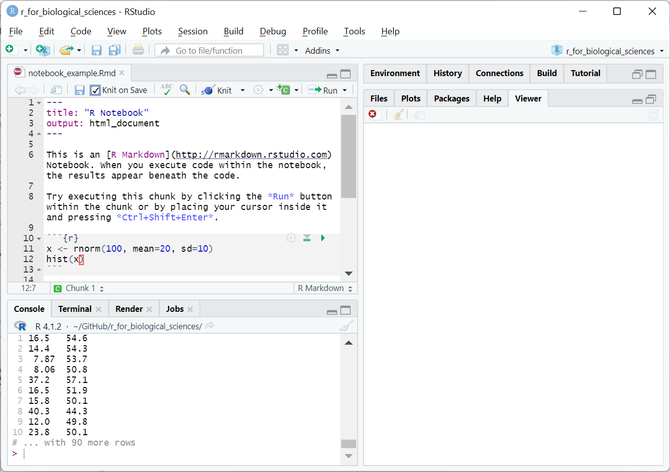
RStudio has full RMarkdown integration to make writing RMarkdown notebooks very easy. Below is a screenshot of an RMarkdown document loaded in RStudio:

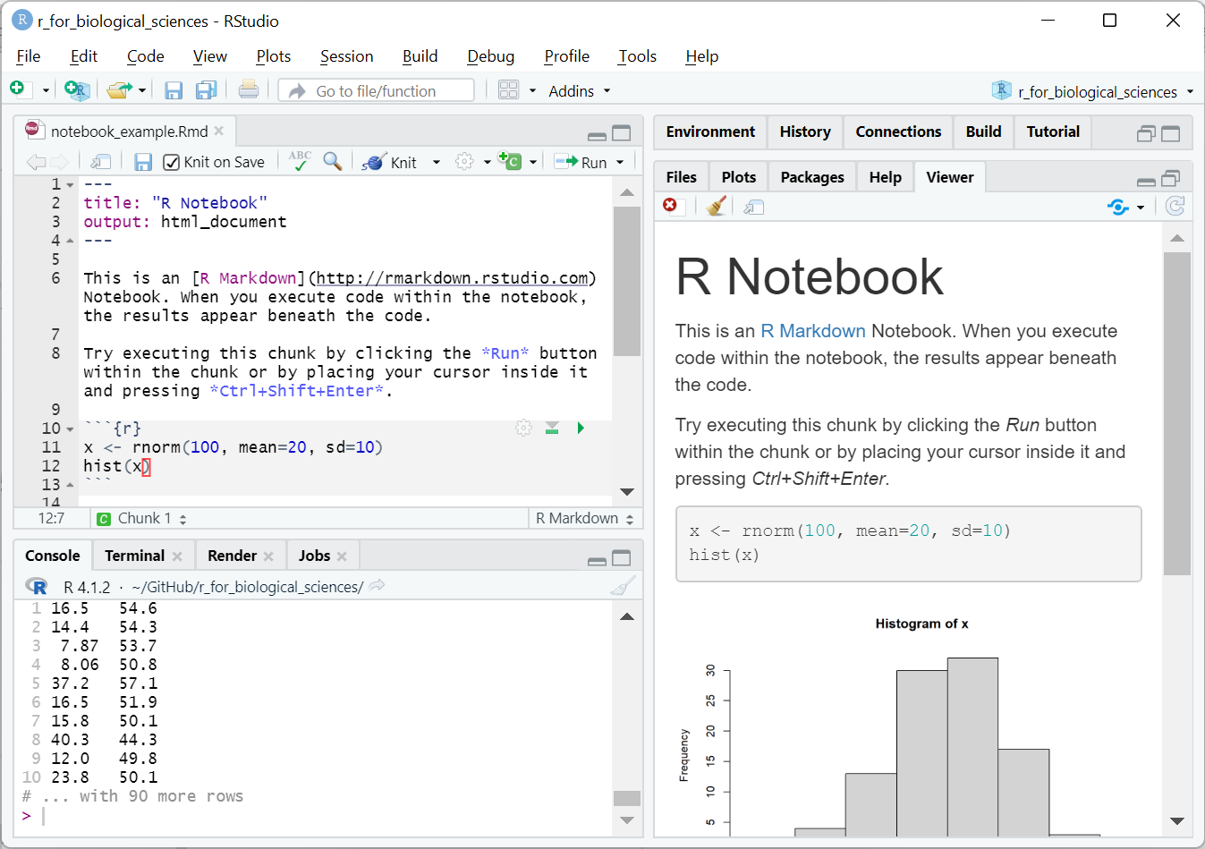
The grey lines starting with ```{r} define a special code block that contains R code that should be executed and the output placed after the block. When run, RStudio will show you the output of the notebook within its interface:

Notice how there is now a plot in the rendered document on the right. The code within the block was run, the plot generated, and inserted into the report. In this case, the notebook created an HTML document that RStudio knows how to display, but could also be opened in a standard web browser.

These blocks are not standard R syntax, but are instead understood and processed by the knitr R package. As the name suggests, the process of generating a report from an RMarkdown document is called “knitting”; you would ask RStudio to knit your RMarkdown into a report.

RMarkdown documents can be knitted into many different formats, including HTML, PDF, Microsoft Word, and even some slide presentation formats. When exporting to HTML, the report may include interactive elements including plots, collapsible sections, and code blocks, and maps.

RMarkdown documents can also be written to accept parameters. This means you can write a single RMarkdown document that can be run on different inputs. Reports for standardized analytical pipelines, as are often implemented by high throughput sequencing cores, can thus be generated trivially for new datasets as they are generated without writing any additional code.