- Syllabus
- 1 Introduction
- 2 Data in Biology
- 3 Preliminaries
- 4 R Programming
- 4.1 Before you begin
- 4.2 Introduction
- 4.3 R Syntax Basics
- 4.4 Basic Types of Values
- 4.5 Data Structures
- 4.6 Logical Tests and Comparators
- 4.7 Functions
- 4.8 Iteration
- 4.9 Installing Packages
- 4.10 Saving and Loading R Data
- 4.11 Troubleshooting and Debugging
- 4.12 Coding Style and Conventions
- 4.12.1 Is my code correct?
- 4.12.2 Does my code follow the DRY principle?
- 4.12.3 Did I choose concise but descriptive variable and function names?
- 4.12.4 Did I use indentation and naming conventions consistently throughout my code?
- 4.12.5 Did I write comments, especially when what the code does is not obvious?
- 4.12.6 How easy would it be for someone else to understand my code?
- 4.12.7 Is my code easy to maintain/change?
- 4.12.8 The
stylerpackage
- 5 Data Wrangling
- 6 Data Science
- 7 Data Visualization
- 8 Biology & Bioinformatics
- 8.1 R in Biology
- 8.2 Biological Data Overview
- 8.3 Bioconductor
- 8.4 Microarrays
- 8.5 High Throughput Sequencing
- 8.6 Gene Identifiers
- 8.7 Gene Expression
- 8.7.1 Gene Expression Data in Bioconductor
- 8.7.2 Differential Expression Analysis
- 8.7.3 Microarray Gene Expression Data
- 8.7.4 Differential Expression: Microarrays (limma)
- 8.7.5 RNASeq
- 8.7.6 RNASeq Gene Expression Data
- 8.7.7 Filtering Counts
- 8.7.8 Count Distributions
- 8.7.9 Differential Expression: RNASeq
- 8.8 Gene Set Enrichment Analysis
- 8.9 Biological Networks .
- 9 EngineeRing
- 10 RShiny
- 11 Communicating with R
- 12 Contribution Guide
- Assignments
- Assignment Format
- Starting an Assignment
- Assignment 1
- Assignment 2
- Assignment 3
- Problem Statement
- Learning Objectives
- Skill List
- Background on Microarrays
- Background on Principal Component Analysis
- Marisa et al. Gene Expression Classification of Colon Cancer into Molecular Subtypes: Characterization, Validation, and Prognostic Value. PLoS Medicine, May 2013. PMID: 23700391
- Scaling data using R
scale() - Proportion of variance explained
- Plotting and visualization of PCA
- Hierarchical Clustering and Heatmaps
- References
- Assignment 4
- Assignment 5
- Problem Statement
- Learning Objectives
- Skill List
- DESeq2 Background
- Generating a counts matrix
- Prefiltering Counts matrix
- Median-of-ratios normalization
- DESeq2 preparation
- O’Meara et al. Transcriptional Reversion of Cardiac Myocyte Fate During Mammalian Cardiac Regeneration. Circ Res. Feb 2015. PMID: 25477501l
- 1. Reading and subsetting the data from verse_counts.tsv and sample_metadata.csv
- 2. Running DESeq2
- 3. Annotating results to construct a labeled volcano plot
- 4. Diagnostic plot of the raw p-values for all genes
- 5. Plotting the LogFoldChanges for differentially expressed genes
- The choice of FDR cutoff depends on cost
- 6. Plotting the normalized counts of differentially expressed genes
- 7. Volcano Plot to visualize differential expression results
- 8. Running fgsea vignette
- 9. Plotting the top ten positive NES and top ten negative NES pathways
- References
- Assignment 6
- Assignment 7
- Appendix
- A Class Outlines
4.7 Functions
Just as a variable is a symbolic representation of a value, a function is a
symbolic representation of code. In other words, a function allows you to
substitute a short name, e.g. mean, for a set of operations on a given input,
e.g. the sum of a set of numbers divided by the number of numbers. R provides a
very large number of functions for common operations in
its default environment, and more functions are provided by packages you can
install separately.
Encapsulating many lines of code into a function is useful for (at least) five distinct reasons:
- Make your code more concise and readable
- Allow you to avoid writing the same code over and over (i.e. reuse it)
- Allow you to systematically test pieces of your code to make sure they do what you intend
- Allow you to share your code easily with others
- Program using a functional programming style (see note box below)
At its core, R is a functional programming language. The details of what this means are outside the scope of this book, but as the name implies this refers to the language being structured around the use of functions. While this property has technical implications on the structure of the language, a more important consequence is the style of programming it entails. The functional programming style (or paradigm) has many advantages, including generally producing programs that are more concise, predictable, provably correct, and performant. provides a good starting point for learning about functional programming.
In order to do anything useful, a function must generally be able to accept
and execute on different inputs; e.g. the mean function wouldn’t be very
useful if it didn’t accept a value! The terminology used in R and many other
programming languages for this is the function must accept or allow you to
pass it arguments. In R, functions accept arguments using the following
*pattern:
# a basic function signature
function_name(arg1, arg2) # function accepts exactly 2 arguments
Here, arg1 and arg2 are formal arguments or named arguments, indicating
this function accepts two arguments. The name of the function (i.e.
function_name) and the pattern of arguments it accepts is called the
function’s signature. Every function has at least one signature, and it is
critical to understand it in order to use the function properly.
In the above example, arg1 and arg2 are required arguments. This means
that the function will not execute without exactly two arguments provided and
will raise an error if you try otherwise:
mean() # compute the arithmetic mean, but of what?
Error in mean.default() : argument "x" is missing, with no default
How do you know what arguments a function requires? All functions provided by
base R and many other packages include detailed documentation that can be
accessed directly through RStudio using either the ? or help():
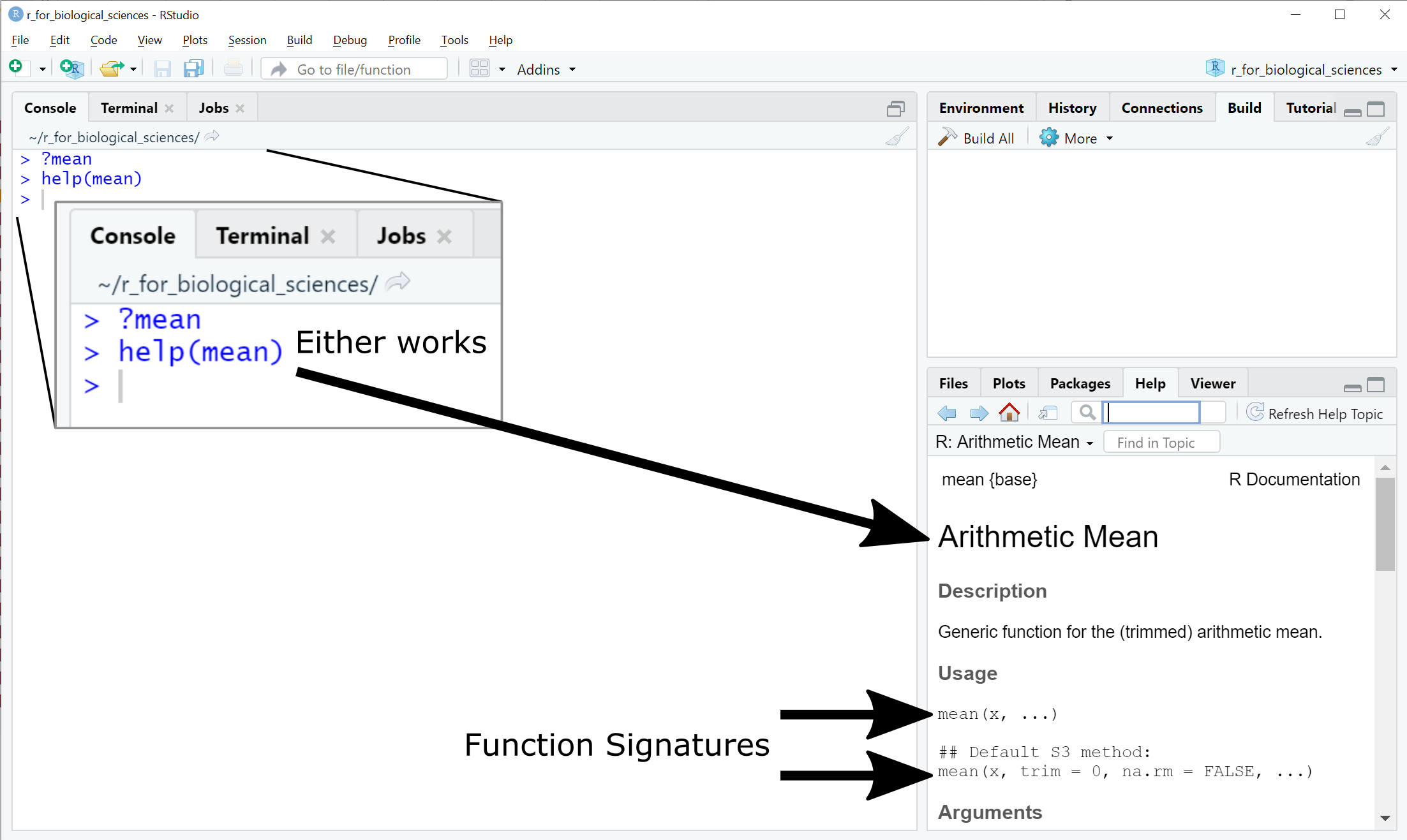
RStudio - help and function signatures
The second signature of the mean function introduces two new types of syntax:
Default argument values - e.g. trim = 0. These are formal arguments that
have a default value if not provided explicitly.
Variable arguments - .... This means the mean function can accept
arguments that are not explicitly listed in the signature. This syntax is called
dynamic dots.
With these definitions, we can now understand the Arguments section of the help documentation:
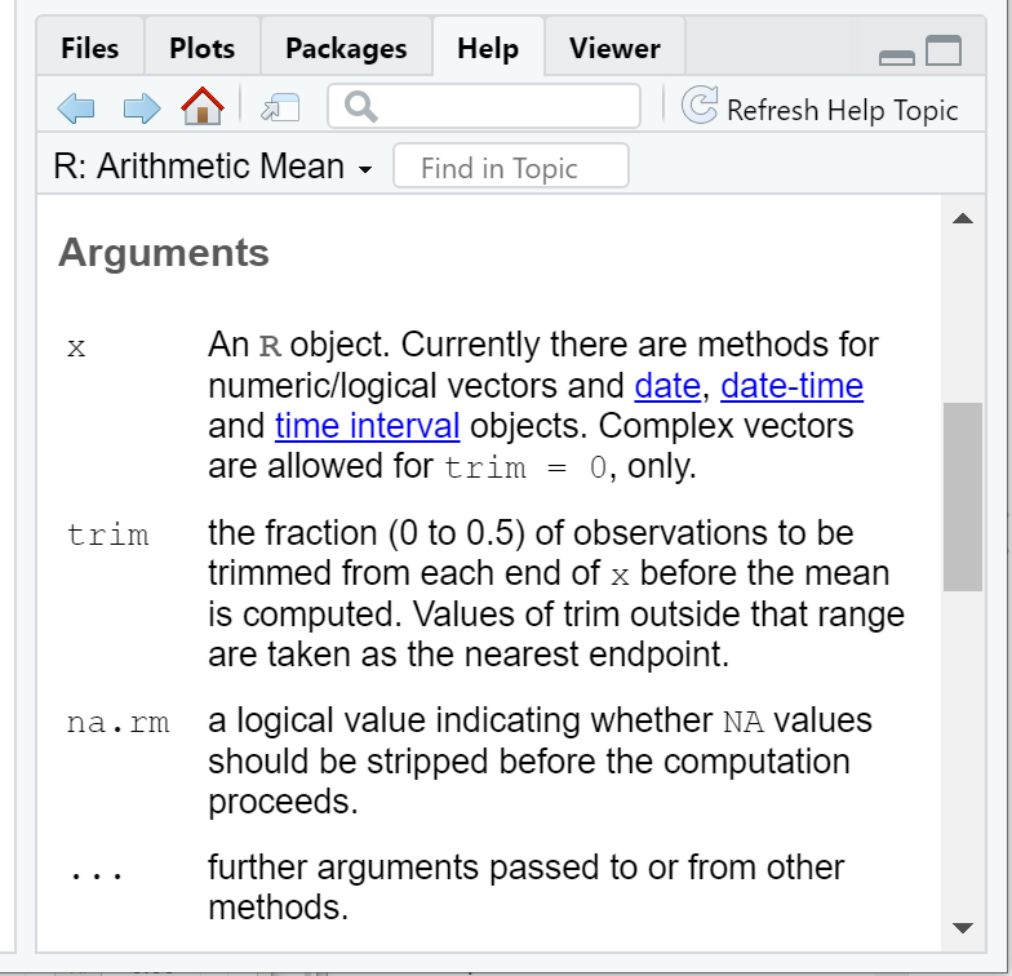
Arguments to the mean function
In other words:
xis the vector of values (more on this in the next section on data structures) we wish to compute the arithmetic mean fortrimis a fraction (i.e. a number between 0 and 0.5) that instructs R to remove a portion of the largest and smallest values fromxprior to computing the mean.na.rmis a logical value (i.e. eitherTRUEorFALSE) that instructs R to removeNAvalues fromxbefore computing the mean.
All function arguments can be specified by name, regardless of whether there is
a default value or not. For instance, the following two mean calls are
equivalent:
# this generates 100 normally distributed samples with mean 0 and standard deviation 1
my_vals <- rnorm(100,mean=0,sd=1)
mean(my_vals)
[1] -0.05826857
mean(x=my_vals)
[1] -0.05826857
To borrow from the Zen of Python, “Explicit is better than implicit.” Being explicit about which variables are being passed as which arguments will almost always make your code easier to read and more likely to do what you intend.
The ... argument catchall can be very dangerous. It allows you to provide
arguments to a function that have no meaning, and R will not raise an error.
Consider the following call to mean:
# this generates 100 normally distributed samples with mean 0 and standard deviation 1
my_vals <- rnorm(100,mean=0,sd=1)
mean(x=my_vals,tirm=0.1)
[1] -0.05826857
Did you spot the mistake? The trim argument name has been misspelled as
tirm, but R did not report an error. Compare the value of mean without the
typo:
mean(x=my_vals,trim=0.1)
[1]-0.02139839
The value we get is different, because R recognizes trim but not tirm and
changes its behavior accordingly. Not all functions have the ... catchall in
their signatures, but many do and so you must be diligent when supplying
arguments to function calls!
4.7.1 DRY: Don’t Repeat Yourself
Sometimes you will find yourself writing the same code more than once to perform the same operation on different data. For example, one common data transformation is standardization or normalization which entails taking a series of numbers, subtracting the mean of all the numbers from them, and dividing each by the standard deviation of the numbers:
# 100 normally distributed samples with mean 20 and standard deviation 10
my_vals <- rnorm(100,mean=20,sd=10)
my_vals_norm <- (my_vals - mean(my_vals))/sd(my_vals)
mean(my_vals_norm)
[1] 0
sd(my_vals_norm)
[1] 1
Later in your code, you may need to standardize a different set of values, so you decide to copy and paste your code from above and replace the variable name to reflect the new data:
# new samples with mean 40 and standard deviation 5
my_other_vals <- rnorm(100,mean=40,sd=5)
my_other_vals_norm <- (my_other_vals - mean(my_other_vals))/sd(my_vals)
mean(my_other_vals_norm)
[1] 0
sd(my_other_vals_norm) # this should be 1!
[1] 0.52351
Notice the mistake? We forgot to change the variable name my_vals to
my_other_vals in our pasted code, which produced an incorrect result. Good
thing we checked!
In general, if you are copying and pasting code from one part of your script to another, you are repeating yourself and have to do a lot of work to be sure you have modified your copy correctly. Copying and pasting code is tempting from an efficiency standpoint, but introduces may opportunities for (often undetected!) errors.
Don’t Repeat Yourself (DRY) is a principle of software development that emphasizes recognizing and avoiding writing the same code over and over by encapsulating code. In R, this is most easily done with functions. If you notice yourself copying and pasting code, or writing the same pattern of code more than once, this is an excellent opportunity to write your own function and avoid repeating yourself!
4.7.2 Writing your own functions
R allows you to define your own function using the following syntax:
function_name <- function(arg1, arg2, ...) {
  # code that does something with arg1, arg2, etc
  return(some_result)
}
You define the name of your function, the number of arguments it accepts and
their names, and the code within the function, which is also called the function
body. Taking the example above, I would define a function named standardize
that accepts a vector of numbers, subtracts the mean from all the values, and
divides them by the standard deviation:
standardize <- function(x) {
  res <- (x - mean(x))/sd(x)
  return(res)
}

my_vals <- rnorm(100,mean=20,sd=10)
my_vals_std <- standardize(my_vals)
mean(my_vals_std)
[1] 0
sd(my_vals_std)
[1] 1

my_other_vals <- rnorm(100,mean=40,sd=5)
my_other_vals_std <- standardize(my_other_vals)
mean(my_other_vals_std)
[1] 0
sd(my_other_vals_std)
[1] 1
Notice above we are assigning the value of the standardize function to new
variables. In R and other languages, the result of a function is returned when
the function is called; the value returned is called the return value. The
return() function makes it clear what the function is returning.
The return() function is not strictly necessary in R; the result of the last
line of code in the body of a function is returned by default. However, to again
to borrow from the Zen of
Python, “Explicit is better than
implicit.” Being explicit about what a function returns by using the return()
function will make your code less error prone and easier to understand.
4.7.3 Scope
In programming, there is a critically important concept called scope. Every variable and function you define when you program has a scope, which defines where in the rest of your code the variable can be accessed. In R, variables defined outside of a function have universal or top level scope, i.e. they can be accessed from anywhere in your script. However, variables defined inside functions can only be accessed from within that function. For example:
x <- 3
multiply_x_by_two <- function() {
  y <- x*2 # x is not defined as a parameter to the function, but is defined outside the function
  return(y)
}
x
[1] 3
multiply_x_by_two()
[1] 6
y
Error: object 'y' not found
Notice that the variable x is accessible within the function
multiply_x_by_two, but the variable y is not accessible outside that
function. The reason that x is accessible within the function is that
multiply_x_by_two inherits the scope where it is defined, which in this case
is the top level scope of your script, which includes x. The scope of y is
limited to the body of the function between the { } curly braces defining
the function.
Accessing variables within functions from outside the function’s scope is very bad practice! Functions should be as self contained as possible, and any values they need should be passed as parameters. A better way to write the function above would be as follows:
x <- 3
multiply_by_two <- function(x) {
  y <- x*2 # x here is defined as whatever is passed to the function!
  y
}
x
[1] 3
multiply_by_two(6)
[1] 12
x # the value of x in the outer scope remains the same, because the function scope does not modify it
[1] 3
Every variable and function you define is subject to the same scope rules above. Scope is a critical concept to understand when programming, and grasping how it works will make your code more predictable and less error prone.