6 Data Wrangling

6.1 The Tidyverse

The tidyverse is “an opinionated collection of R packages designed for data science.” The packages are all designed to work together with a unified approach that helps code look consistent and neat. In the opinion of this author, the tidyverse practically changes the R language from a principally statistical programming language into an efficient and expressive data science language. While it is still important to understand the language fundamentals presented in our chapter on the R programming language, the tidyverse uses a distinct set of coding conventions that lets it achieve greater expressiveness, conciseness, and correctness relative to the base R language.

As a data science language, R+tidyverse (referred to as simply tidyverse in this book) is strongly focused on operations related to loading, manipulating, visualizing, summarizing, and analyzing data sets from many domains. While this is a major strength of tidyverse and its community, it means that many educational materials are written for this general use case, and not for those practicing biological data analysis. While the general data manipulation operations are often the same between biological data analysis and these general case examples, biological analysis practitioners must nonetheless translate concepts from these general cases to the common data analysis tasks they must perform. Some analytical patterns are more common in biological data analysis than others, so these materials focus on that subset of operations in this book to aid the learning in applying the concepts to their problems as directly as possible.

6.2 Tidyverse Basics

Since tidyverse is a set of packages that work together, you will often want to load multiple packages at the same time. The tidyverse authors recognize this, and defined a set of reasonable packages to load at once when loading the metapackage (i.e. a package that contains multiple packages):

library(tidyverse)
-- Attaching packages --------------------------------------------- tidyverse 1.3.1 --
v ggplot2 3.3.5     v purrr   0.3.4
v tibble  3.1.6     v dplyr   1.0.7
v tidyr   1.1.4     v stringr 1.4.0
v readr   2.1.1     v forcats 0.5.1
-- Conflicts ------------------------------------------------ tidyverse_conflicts() --
x dplyr::filter() masks stats::filter()
x dplyr::lag()    masks stats::lag()

The packages in the Attaching packages section are those loaded by default, and each of these packages adds a unique set of functions to your R environment. We will mention functions from many of these packages as we go through this chapter, but for now here is a table of these packages and briefly what they do:

Package	Description
ggplot2	Plotting using the grammar of graphics
tibble	Simple and sane data frames
tidyr	Operations for making data “tidy”
readr	Read rectangular text data into tidyverse
purrr	Functional programming tools for tidyverse
dplyr	“A Grammar of Data Manipulation”
stringr	Makes working with strings in R easier
forcats	Operations for using categorical variables

Notice the dplyr::filter() syntax in the Conflicts section. filter is defined as a function in both the dplyr package as well as the base R stats package. The stats package is loaded by default when you run R, and thus the filter function is defined (specifically, it performs linear filtering on time series data). However, when dplyr is loaded, it also has a filter function which overrides the definition from the stats package. This is why the tidyverse package reports this as a conflict when loaded:

-- Conflicts ------------------------------------------------ tidyverse_conflicts() --
x dplyr::filter() masks stats::filter()

This is tidyverse telling you that the filter function has been redefined and you should make sure you are aware of that.

However, if you did want to use the original stats defined filter function, you may still access it using the :: namespace operator. This operator lets you “look inside” a loaded package, for example dplyr, and access a function within the namespace of that package:

library(dplyr)
# the filter() function definition is now from the dplyr package, and not from the stats package
# the following two lines of code execute the same function
filter(df)
dplyr::filter(df)
# to access the stats definition of the filter function, use the namespace operator
stats::filter(df)

Most functions defined by a package can be accessed using the :: operator, and it is often a good idea to do so, to ensure you are calling the right function.

6.3 Importing Data

The first operation we typically must perform when analyzing data is reading our data from a file into R. The readr package in the default tidyverse packages contains the following similar functions that import data from delimited text files:

Function	Brief description/use
`read_csv`	Delimiter: `,` - Decimal separator: `.`
`read_csv2`	Delimiter: `;` - Decimal separator: `,`
`read_tsv`	Delimiter: `<tab>` - Decimal separator: `.`
`read_delim`	Delimiter: set by user - Decimal separator: `.`

Some CSV files can be very large and may be compressed to save space. There are many different file compression algorithms, but the most common in data science and biology are gzip and bzip. All the readr file reading functions can work with compressed files directly, so you do not need to decompress them first.

Each of these functions returns a special data frame called a tibble, which is explained in the next section.

Note that readr also has functions for writing delimited files. These functions behave similarly to the read_X functions but instead of creating a tibble from a file, they create a file from a tibble. You will frequently need to export the results of your analysis to share with collaborators and also as part of larger workflows that use tools other than R.

6.4 The tibble

Data in tidyverse is organized primarily in a special data frame object called a tibble. The tibble() function is defined in the tibble package of the tidyverse:

library(tibble) # or
library(tidyverse)
tbl <- tibble(
    x = rnorm(100, mean=20, sd=10),
    y = rnorm(100, mean=50, sd=5)
)
tbl
# A tibble: 100 x 2
       x     y
   <dbl> <dbl>
 1 16.5   54.6
 2 14.4   54.3
 3  7.87  53.7
 4  8.06  50.8
 5 37.2   57.1
 6 16.5   51.9
 7 15.8   50.1
 8 40.3   44.3
 9 12.0   49.8
10 23.8   50.1
# ... with 90 more rows

A tibble stores rectangular data, i.e. a grid of data elements with where every column has the same number of rows. You can access individual columns in the same way as with base R data frames:

tbl$x
[1] 29.572549 12.015877 15.235536 23.071761 32.254703 48.048651 21.905756
[8] 15.511768 34.872685 21.352433 12.515230 23.608096  6.778630 12.342237
...
tbl[1,"x"] # access the first element of x
# A tibble: 1 x 1
    x
  <dbl>
1  29.6
tbl$x[1]
[1] 29.57255

tibbles (and regular data frames) typically have names for their columns. In the above example, the column names are x and y, accessed using the colnames function:

colnames(tbl)
[1] "x" "y"

Column names may be changed using this same function:

colnames(tbl) <- c("a","b")
tbl
# A tibble: 100 x 2
       a     b
   <dbl> <dbl>
 1 16.5   54.6
 2 14.4   54.3
 3  7.87  53.7
 4  8.06  50.8
 5 37.2   57.1
 6 16.5   51.9
 7 15.8   50.1
 8 40.3   44.3
 9 12.0   49.8
10 23.8   50.1
# ... with 90 more rows

As we will see again later, we can also use dplyr::rename to rename columns as well:

dplyr::rename(tbl,
  a = x,
  b = y
)

tibbles and dataframes also have row names as well as column names:

rownames(tbl)
[1] "1" "2" "3"...

However, the tibble support for row names is only included for compatibility with base R data frames and should generally be avoided. The reason is that row names are basically a character column that has different semantics than every other column, and the authors of tidyverse believe row names are better stored as a normal column.

tibble - working with row names

The tibble package provides a convenient way to construct simple tibbles manually with the tribble() function, which stands for “transposed tibble”:

gene_stats <- tribble(
    ~gene, ~test1_stat, ~test1_p, ~test2_stat, ~test2_p,
   "apoe", 12.509293,   0.1032,   34.239521,   1.3e-5,
   "hoxd1",  4.399211,   0.6323,   16.332318,   0.0421,
   "snca", 45.748431,   4.2e-9,    0.757188,   0.9146,
)
gene_stats

## # A tibble: 3 × 5
##   gene  test1_stat      test1_p test2_stat  test2_p
##   <chr>      <dbl>        <dbl>      <dbl>    <dbl>
## 1 apoe       12.5  0.103            34.2   0.000013
## 2 hoxd1       4.40 0.632            16.3   0.0421  
## 3 snca       45.7  0.0000000042      0.757 0.915

This made-up dataset includes statistics and p-values from two different statistical tests (again, made up) for three human genes. We will use this example below in the Arranging Data section.

6.5 Tidy Data

The tidyverse packages are designed to operate with so-called “tidy data”. From the tidy data section of the R for Data Science book, the following rules make data tidy:

Each variable must have its own column.
Each observation must have its own row.
Each value must have its own cell.

Here, a variable is a quantity or property that every observation in our dataset has, and each observation is a separate instance of those variable (e.g. a different sample, subject, etc). In our gene_stats example tibble above, the columns referring to different test statistics are the variables, and each gene in each row is an “observation”, and each cell has a value; we can therefore say that the dataset is tidy:

gene_stats

## # A tibble: 3 × 5
##   gene  test1_stat      test1_p test2_stat  test2_p
##   <chr>      <dbl>        <dbl>      <dbl>    <dbl>
## 1 apoe       12.5  0.103            34.2   0.000013
## 2 hoxd1       4.40 0.632            16.3   0.0421  
## 3 snca       45.7  0.0000000042      0.757 0.915

Each row being an “observation” is somewhat abstract in this case; we could say that we “observed” the same test for all the genes in the tibble. Depending on what dataset we are working with, we sometimes have to be flexible in our conceptualization of what constitutes variables and observations.

The R for Data Science book depicts these rules in the following illustration:

Tidy data - from R for Data Science

These rules are pretty generic, and in general a dataset might require some work to manipulate it into tidy form. Fortunately for those of us working in biology and bioinformatics, very many of our datasets are already provided in a format that is very close to being tidy, or the tools we use to process biological data do so for us. For this reason, details about the tidying operations that might be needed for data in the general case are left for reading in the tidy data section of R for Data Science book.

There is one very big and common exception to the claim above that biological data is usually already tidy that. Briefly, from the illustration above, tidy data has observations as rows and variables as columns. However, the datasets that we often use, e.g. gene expression matrices, are organized to have variables (e.g. genes) as rows and observations (e.g. samples) as columns. This means some operations to summarize variables across observations, which are very common to compute, are not easily done with the tidyverse functions like mutate(). We describe how to work around this difference in the section Biological data is NOT Tidy!.

Tidy data - R for Data Science

6.6 pipes

One of the key tidyverse programming patterns is chaining manipulations of tibbles together using the %>% operator. We very often want to perform serial operations on a data frame, for example read in a file, rename one of the columns, subset the rows based on some criteria, and compute summary statistics on the result. We might implement such operations using a variable and assignment:

# data_file.csv has two columns: bad_cOlumn_name and numeric_column
data <- readr::read_csv("data_file.csv")
data <- dplyr::rename(data, "better_column_name"=bad_cOlumn_name)
data <- dplyr::filter(data, better_column_name %in% c("condA","condB"))
data_grouped <- dplyr::group_by(data, better_column_name)
summarized <- dplyr::summarize(data_grouped, mean(numeric_column))

The repeated use of data and the intermediate data_grouped variable may be unnecessary if you’re only interested in the summarized result. The code is also not very straightforward to read. Using the %>% operator, we can write the same sequence of operations in a much more concise manner:

data <- readr::read_csv("data_file.csv") %>%
      dplyr::rename("better_column_name"=bad_cOlumn_name) %>%
      dplyr::filter(better_column_name %in% c("condA","condB")) %>%
      dplyr::group_by(better_column_name) %>%
      dplyr::summarize(mean(numeric_column))

Note that the function calls in the piped example do not have the data variable passed in explicitly. This is because the %>% operator passes the result of the function immediately preceding it as the first argument to the next function automatically. This convention allows us to focus on writing only the important parts of the code that perform the logic of our analysis, and avoid unnecessary and potentially distracting additional characters that make the code less readable.

6.7 Arranging Data

After we have loaded our data from a file into a tibble, we often need to manipulate it in various ways to make the values amenable to our desired analysis. Such manipulations might include renaming poorly named columns, filtering out certain records, deriving new columns using the values in others, changing the order of rows etc. These operations may collectively be termed arranging the data and many are provided in the *dplyr package. We will cover some of the most common data arranging functions here, but there are many more in the dplyr package worth knowing.

In the examples below, we will make use of the following made-up tibble that contains fake statistics and p-values for three human genes:

gene_stats

## # A tibble: 3 × 5
##   gene  test1_stat      test1_p test2_stat  test2_p
##   <chr>      <dbl>        <dbl>      <dbl>    <dbl>
## 1 apoe       12.5  0.103            34.2   0.000013
## 2 hoxd1       4.40 0.632            16.3   0.0421  
## 3 snca       45.7  0.0000000042      0.757 0.915

The gene_stats tibble above is a simple example of a very common type of data we work with in biology; namely instead of raw data, we work with statistics that have been computed using raw data that help us interpret the results. While these statistics may not be ‘data’ per se, we can still use all the functions and strategies in the tidyverse to work with them.

The tidyverse is a very big place. RStudio created many helpful cheatsheets to aid in looking up how do to certain operations. The cheatsheet on dplyr has lots of useful information on how to use the many functions in the package.

6.7.1 `dplyr::mutate()` - Create new columns using other columns

Many biological analysis procedures perform some kind of statistical test on a collection of features (e.g. genes) and produce p-values that indicate how “surprising” each feature is according to the test. The p-values in our tibble are nominal, i.e. they have not been adjusted for multiple hypotheses. Briefly, when we run multiple tests like we are on each of our three genes, there is a chance that some of the tests will have a small p-value simply by chance. Multiple testing correction procedures adjust nominal p-values to account for this possibility in a number of different ways, but the most common procedure in biological analysis is the Benjamini-Hochberg or False Discovery Rate (FDR) procedure. In R, the p.adjust function can perform several of these procedures, including FDR:

dplyr::mutate(gene_stats,
  test1_padj=p.adjust(test1_p,method="fdr")
)

## # A tibble: 3 × 6
##   gene  test1_stat      test1_p test2_stat  test2_p   test1_padj
##   <chr>      <dbl>        <dbl>      <dbl>    <dbl>        <dbl>
## 1 apoe       12.5  0.103            34.2   0.000013 0.155       
## 2 hoxd1       4.40 0.632            16.3   0.0421   0.632       
## 3 snca       45.7  0.0000000042      0.757 0.915    0.0000000126

Notice how the adjusted p-values are larger than the nominal ones; this is the effect of the multiple testing procedure. Since we have two sets of p-values, we must compute the FDR on each of them, which we can do in the same call to mutate():

gene_stats_mutated <- dplyr::mutate(gene_stats,
  test1_padj=p.adjust(test1_p,method="fdr"),
  test2_padj=p.adjust(test2_p,method="fdr")
)
gene_stats_mutated

## # A tibble: 3 × 7
##   gene  test1_stat      test1_p test2_stat  test2_p   test1_padj test2_padj
##   <chr>      <dbl>        <dbl>      <dbl>    <dbl>        <dbl>      <dbl>
## 1 apoe       12.5  0.103            34.2   0.000013 0.155          0.000039
## 2 hoxd1       4.40 0.632            16.3   0.0421   0.632          0.0632  
## 3 snca       45.7  0.0000000042      0.757 0.915    0.0000000126   0.915

Another common operation is to create new columns derived from the values in multiple other columns. We (or our wetlab colleagues) might decide it is convenient to have a new column with TRUE or FALSE based on whether the gene was significant in either test. Such a column would make it easy to filter genes down to just ones that might be interesting in tools like Excel. We can create new columns from multiple columns just as easily using the mutate() function:

dplyr::mutate(gene_stats_mutated,
  signif_either=(test1_padj < 0.05 | test2_padj < 0.05),
  signif_both=(test1_padj < 0.05 & test2_padj < 0.05)
)

## # A tibble: 3 × 9
##   gene  test1_stat      test1_p test2_stat  test2_p   test1_padj test2_padj
##   <chr>      <dbl>        <dbl>      <dbl>    <dbl>        <dbl>      <dbl>
## 1 apoe       12.5  0.103            34.2   0.000013 0.155          0.000039
## 2 hoxd1       4.40 0.632            16.3   0.0421   0.632          0.0632  
## 3 snca       45.7  0.0000000042      0.757 0.915    0.0000000126   0.915   
## # ℹ 2 more variables: signif_either <lgl>, signif_both <lgl>

Recall that the | and & operators execute ‘or’ and ‘and’ logic, respectively. The above example required the creation of a new variable gene_stats_mutated because the columns test1_padj and test2_padj need to be in the tibble before computing the new fields. However, in mutate(), columns created first in the function call are available to later columns. In the following example, note that test1_padj is created first and then used to create the signif columns:

dplyr::mutate(gene_stats,
  test1_padj=p.adjust(test1_p,method="fdr"), # test1_padj created
  test2_padj=p.adjust(test2_p,method="fdr"),
  signif_either=(test1_padj < 0.05 | test2_padj < 0.05), #test1_padj used
  signif_both=(test1_padj < 0.05 & test2_padj < 0.05)
)

## # A tibble: 3 × 9
##   gene  test1_stat      test1_p test2_stat  test2_p   test1_padj test2_padj
##   <chr>      <dbl>        <dbl>      <dbl>    <dbl>        <dbl>      <dbl>
## 1 apoe       12.5  0.103            34.2   0.000013 0.155          0.000039
## 2 hoxd1       4.40 0.632            16.3   0.0421   0.632          0.0632  
## 3 snca       45.7  0.0000000042      0.757 0.915    0.0000000126   0.915   
## # ℹ 2 more variables: signif_either <lgl>, signif_both <lgl>

The alternative would be to split this into two mutate() commands, the first creating the adjusted p-value columns and the second creating the significance columns. dplyr recognizes how common it is to build new variables off of other new variables in a mutate() command, and therefore provides this convenient behavior.

mutate() can also be used to modify columns in place. The official convention for human gene symbols is that they are upper case, but for some reason our tibble contains lower case gene symbols. We can correct this using mutate() but first we should talk about the stringr package which makes working with strings much easier than with base R functions.

6.7.2 `stringr` - Working with character values

Base R does not have very convenient functions for working with character strings (or just strings). This is due to its original intent a statistical programming language, where string manipulation is not (in principle) a common operation. However, in practice, we must frequently manipulate strings while loading, cleaning, and analyzing datasets. The stringr package aims to make working with strings “as easy as possible.”

The package includes many useful functions for operating on strings, including searching for patterns, mutating strings, lexicographical sorting, combining multiple strings together (i.e. concatenation), and performing complex search/replace operations. There are far too many useful functions to cover here and you should become comfortable reading the stringr documentation and the very helpful stringr cheatsheet.

In the previous section, we noted that the gene symbols in our tibble were lower case while official gene symbols are in upper case. We can use the stringr function stringr::str_to_upper() with the dplyr::mutate() function to perform this adjustment easily:

dplyr::mutate(gene_stats,
  gene=stringr::str_to_upper(gene)
)

## # A tibble: 3 × 5
##   gene  test1_stat      test1_p test2_stat  test2_p
##   <chr>      <dbl>        <dbl>      <dbl>    <dbl>
## 1 APOE       12.5  0.103            34.2   0.000013
## 2 HOXD1       4.40 0.632            16.3   0.0421  
## 3 SNCA       45.7  0.0000000042      0.757 0.915

Now are gene symbols have the appropriate case, and our wetlab colleagues won’t complain about it. :)

6.7.2.1 Regular expressions

Many of the string operations in the stringr package use regular expression syntax. A regular expression is a sequence of characters that describes patterns in text. Regular expressions are written in a sort of mini programming language where certain characters have special meaning that help in defining search patterns that identifies the location of sequences of characters in text that follow a particular pattern specified by the regular expression. This is similar to the “Find” functionality in many word processors, but is more powerful due to the flexibility of the patterns that can be found.

A simple example will be helpful. Let’s say we have a tibble containing the result of a (made-up) statistical test for all the genes in a genome:

de_genes

## # A tibble: 40,982 × 4
##    hgnc_symbol   mean         p    padj
##    <chr>        <int>     <dbl>   <dbl>
##  1 MT-TF          445 0.0121    0.0206 
##  2 MT-RNR1        877 0.00257   0.0114 
##  3 MT-TV           45 0.0308    0.0373 
##  4 MT-RNR2        703 0.00211   0.0110 
##  5 MT-TL1         589 0.00125   0.00990
##  6 MT-ND1      674882 0.0000105 0.00583
##  7 MT-TI            6 0.0743    0.0788 
##  8 MT-TQ         1393 0.00436   0.0135 
##  9 MT-TM          321 0.0112    0.0198 
## 10 MT-ND2         650 0.00494   0.0141 
## # ℹ 40,972 more rows

Now let’s say we’re interested in examining the results for the BRCA family of genes, BRCA1 and BRCA2. We can use filter() on the data frame to look for them individually:

de_genes %>% filter(hgnc_symbol == "BRCA1" | hgnc_symbol == "BRCA2")

## # A tibble: 2 × 4
##   hgnc_symbol  mean       p   padj
##   <chr>       <int>   <dbl>  <dbl>
## 1 BRCA2        1104 0.00660 0.0157
## 2 BRCA1           5 0.141   0.144

This isn’t so bad, but we can do the same thing with stringr::str_detect() , which returns TRUE if the provided pattern matches the input and FALSE otherwise, a regular expression, and the [dplyr::filter() function], which is described in greater detail in a later section:

dplyr::filter(de_genes, str_detect(hgnc_symbol,"^BRCA[12]$"))

## # A tibble: 2 × 4
##   hgnc_symbol  mean       p   padj
##   <chr>       <int>   <dbl>  <dbl>
## 1 BRCA2        1104 0.00660 0.0157
## 2 BRCA1           5 0.141   0.144

The argument "^BRCA[12]$" is a regular expression that searches for the following:

Search for genes that start with the characters BRCA - the ^ at the beginning of the pattern stands for the start of the string
For genes that start with BRCA, then look for genes where the next character is either 1 or 2 with [12] - the characters between the [] are searched for explicitly, and any character encountered that is not listed between them results in a non-match
For genes that start with BRCA followed with either a 1 or a 2, match successfully if the number is at the end of the name - the $ at the end of the pattern stands for the end of the string

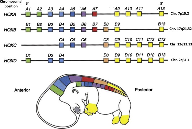
We can use these principles to find genes with more complex naming conventions. The Homeobox (HOX) genes encode DNA binding proteins that regulate gene expression of genes involved in morphgenesis and cell differentiation in vertebrates. In humans, HOX genes are organized into 4 clusters of paralogs that were the result of three DNA duplication events in the distant evolutionary past(Abbasi 2015), where each cluster encodes a subset of 13 distinct HOX genes placed next to each other. Each of these clusters has been assigned a letter identifier A-D (e.g. HOXA, HOXB, HOXC, and HOXD) and each paralogous gene within each cluster is assigned the same number (e.g. HOXA4, HOXB4, HOXC4, and HOXD4 are paralogs). There are 13 HOX genes in total, though not all genes remain in all clusters (e.g. HOXA1, HOXB1, and HOXD1 exist but HOXC1 was lost over time). The following figure depicts the human HOX gene clusters:

Human HOX gene clusters - Veraksa, A.; Del Campo, M.; McGinnis, W. Developmental Patterning Genes and their Conserved Functions: From Model Organisms to Humans. Mol. Genet. Metab. 2000, 69 (2), 85–100.

Let’s say we want to extract out all the HOX genes from our gene statistics. We can write a regular expression that matches the pattern described above:

dplyr::filter(de_genes, str_detect(hgnc_symbol,"^HOX[A-D][0-9]+$")) %>%
  dplyr::arrange(hgnc_symbol)

## # A tibble: 39 × 4
##    hgnc_symbol  mean        p    padj
##    <chr>       <int>    <dbl>   <dbl>
##  1 HOXA1          46 0.0443   0.0499 
##  2 HOXA10        255 0.0215   0.0289 
##  3 HOXA11        300 0.00947  0.0182 
##  4 HOXA13       1343 0.00425  0.0134 
##  5 HOXA2         232 0.0162   0.0241 
##  6 HOXA3          62 0.0280   0.0348 
##  7 HOXA4        1124 0.00648  0.0156 
##  8 HOXA5        2036 0.000764 0.00915
##  9 HOXA6           7 0.100    0.104  
## 10 HOXA7       18721 0.000546 0.00882
## # ℹ 29 more rows

In this query we used two new regular expression features:

within the [] we specified a range of characters A-D and 0-9 which will match any of the characters between A and D (i.e. A, B, C, or D) and 0 and 9 respectively
the + character means “match one or more of the preceding expression”, which in our case is the [0-9]. This allows us to match genes with only a single number (e.g. HOXA1) as well as double digit numbers (e.g. HOXA10).

Since we know the cluster identifier part of the HOX gene names (i.e. the [A-D] part) is exactly one character long, we could alternatively write the regular expression as follows, using the special . character:

dplyr::filter(de_genes, str_detect(hgnc_symbol,"^HOX.[0-9]+$")) %>%
  dplyr::arrange(hgnc_symbol)

## # A tibble: 39 × 4
##    hgnc_symbol  mean        p    padj
##    <chr>       <int>    <dbl>   <dbl>
##  1 HOXA1          46 0.0443   0.0499 
##  2 HOXA10        255 0.0215   0.0289 
##  3 HOXA11        300 0.00947  0.0182 
##  4 HOXA13       1343 0.00425  0.0134 
##  5 HOXA2         232 0.0162   0.0241 
##  6 HOXA3          62 0.0280   0.0348 
##  7 HOXA4        1124 0.00648  0.0156 
##  8 HOXA5        2036 0.000764 0.00915
##  9 HOXA6           7 0.100    0.104  
## 10 HOXA7       18721 0.000546 0.00882
## # ℹ 29 more rows

Here, the . character is interpreted by the regex to match any single character, regardless of what it is, between the HOX part and the number part. This also requires that there exist exactly one character between the two parts; a gene symbol HOX1 would not be matched, because the 1 would match to the ., but no number remains to match to the [0-9]+ part.

Sometimes you want to search text for characters that are considered special in the regular expression language. For example, if you had a list of filenames:

filenames <- tribble(
  ~name,
  "annotation.csv",
  "file1.txt",
  "file2.txt",
  "results.csv"
)

and wanted to limit to just those with the .txt extension, you need to match using a literal . character:

filter(filenames, stringr::str_detect(name,"[.]txt$"))

## # A tibble: 2 × 1
##   name     
##   <chr>    
## 1 file1.txt
## 2 file2.txt

Inside a [], characters do not have their usual regular expression meaning, and therefore [.] will match a literal . character. Instead of using the [] syntax, you may also escape these literal characters using two back slashes:

filter(filenames, stringr::str_detect(name,"\\.txt$"))

## # A tibble: 2 × 1
##   name     
##   <chr>    
## 1 file1.txt
## 2 file2.txt

Regular expressions are very powerful, and can do much more than what is described here. See the regular expression tutorial linked in the readmore box to learn more details.

6.7.3 `dplyr::select()` - Subset Columns by Name

Our mutate() operations above created a number of new columns in our tibble, but we did not specify where in the tibble the new columns should go. Let’s consider the mutated tibble we created with all four new columns:

dplyr::mutate(gene_stats,
  test1_padj=p.adjust(test1_p,method="fdr"),
  test2_padj=p.adjust(test2_p,method="fdr"),
  signif_either=(test1_padj < 0.05 | test2_padj < 0.05),
  signif_both=(test1_padj < 0.05 & test2_padj < 0.05),
  gene=stringr::str_to_upper(gene)
)

## # A tibble: 3 × 9
##   gene  test1_stat      test1_p test2_stat  test2_p   test1_padj test2_padj
##   <chr>      <dbl>        <dbl>      <dbl>    <dbl>        <dbl>      <dbl>
## 1 APOE       12.5  0.103            34.2   0.000013 0.155          0.000039
## 2 HOXD1       4.40 0.632            16.3   0.0421   0.632          0.0632  
## 3 SNCA       45.7  0.0000000042      0.757 0.915    0.0000000126   0.915   
## # ℹ 2 more variables: signif_either <lgl>, signif_both <lgl>

From a readability standpoint, it might be helpful if all the columns that are about each test were grouped together, rather than having to look at the end of the tibble to find them.

The dplyr::select() function allows you to pick specific columns out of a larger tibble in whatever order you choose:

stats <- dplyr::select(gene_stats, test1_stat, test2_stat)
stats

## # A tibble: 3 × 2
##   test1_stat test2_stat
##        <dbl>      <dbl>
## 1      12.5      34.2  
## 2       4.40     16.3  
## 3      45.7       0.757

Here we have explicitly selected the statistics columns. dplyr also has helper functions that allow for more flexible selection of columns. For example, if all of the columns we wished to select ended with _stat, we could use the ends_with() helper function:

stats <- dplyr::select(gene_stats, ends_with("_stat"))
stats

## # A tibble: 3 × 2
##   test1_stat test2_stat
##        <dbl>      <dbl>
## 1      12.5      34.2  
## 2       4.40     16.3  
## 3      45.7       0.757

If you so desire, select() allows for the renaming of selected columns:

stats <- dplyr::select(gene_stats,
  t=test1_stat,
  chisq=test2_stat
)
stats

## # A tibble: 3 × 2
##       t  chisq
##   <dbl>  <dbl>
## 1 12.5  34.2  
## 2  4.40 16.3  
## 3 45.7   0.757

If we knew that these test statistics actually corresponded to some kind of t-test and a $\chi$-squared test, naming the columns of the tibble appropriately may help others (and possibly you) understand your code better.

We can use the dplyr::select() function to obtain our desired column order:

dplyr::mutate(gene_stats,
  test1_padj=p.adjust(test1_p,method="fdr"),
  test2_padj=p.adjust(test2_p,method="fdr"),
  signif_either=(test1_padj < 0.05 | test2_padj < 0.05),
  signif_both=(test1_padj < 0.05 & test2_padj < 0.05),
  gene=stringr::str_to_upper(gene)
) %>%
dplyr::select(
    gene,
    test1_stat, test1_p, test1_padj,
    test2_stat, test2_p, test2_padj,
    signif_either,
    signif_both
)

## # A tibble: 3 × 9
##   gene  test1_stat      test1_p   test1_padj test2_stat  test2_p test2_padj
##   <chr>      <dbl>        <dbl>        <dbl>      <dbl>    <dbl>      <dbl>
## 1 APOE       12.5  0.103        0.155            34.2   0.000013   0.000039
## 2 HOXD1       4.40 0.632        0.632            16.3   0.0421     0.0632  
## 3 SNCA       45.7  0.0000000042 0.0000000126      0.757 0.915      0.915   
## # ℹ 2 more variables: signif_either <lgl>, signif_both <lgl>

Now the order of our columns is clear and convenient. It is not necessary to list the columns for each test statistic on the same line, but the author thinks this makes the code easier to read and understand.

6.7.4 `dplyr::filter()` - Pick rows out of a data set

Often, the first step in interpreting an analysis is to identify the features that are significant at some adjusted p-value threshold. First we will save our mutated tibble to another variable, to aid in demonstration:

gene_stats_mutated <- dplyr::mutate(gene_stats,
  test1_padj=p.adjust(test1_p,method="fdr"),
  test2_padj=p.adjust(test2_p,method="fdr"),
  signif_either=(test1_padj < 0.05 | test2_padj < 0.05),
  signif_both=(test1_padj < 0.05 & test2_padj < 0.05),
  gene=stringr::str_to_upper(gene)
) %>%
dplyr::select(
    gene,
    test1_stat, test1_p, test1_padj,
    test2_stat, test2_p, test2_padj,
    signif_either,
    signif_both
)

Now we can use the dplyr::filter() function to select rows based on whether they are significant in either test this with our above example.

dplyr::filter(gene_stats_mutated, test1_padj < 0.05)

## # A tibble: 1 × 9
##   gene  test1_stat      test1_p   test1_padj test2_stat test2_p test2_padj
##   <chr>      <dbl>        <dbl>        <dbl>      <dbl>   <dbl>      <dbl>
## 1 SNCA        45.7 0.0000000042 0.0000000126      0.757   0.915      0.915
## # ℹ 2 more variables: signif_either <lgl>, signif_both <lgl>

dplyr::filter(gene_stats_mutated, test2_padj < 0.05)

## # A tibble: 1 × 9
##   gene  test1_stat test1_p test1_padj test2_stat  test2_p test2_padj
##   <chr>      <dbl>   <dbl>      <dbl>      <dbl>    <dbl>      <dbl>
## 1 APOE        12.5   0.103      0.155       34.2 0.000013   0.000039
## # ℹ 2 more variables: signif_either <lgl>, signif_both <lgl>

Here we are filtering the result so that only genes with nominal p-value less than 0.05 remain. Note we filter on the two tests separately, but we can also combine these tests using logical operators to achieve different results:

# | means "logical or", meaning the row is retained if either condition is true
dplyr::filter(gene_stats_mutated, test1_padj < 0.05 | test2_padj < 0.05)

## # A tibble: 2 × 9
##   gene  test1_stat      test1_p   test1_padj test2_stat  test2_p test2_padj
##   <chr>      <dbl>        <dbl>        <dbl>      <dbl>    <dbl>      <dbl>
## 1 APOE        12.5 0.103        0.155            34.2   0.000013   0.000039
## 2 SNCA        45.7 0.0000000042 0.0000000126      0.757 0.915      0.915   
## # ℹ 2 more variables: signif_either <lgl>, signif_both <lgl>

Only APOE and SCNA are significant in at least one of the tests.

# & means "logical and", meaning the row is retained only if both conditions are true
dplyr::filter(gene_stats_mutated, test1_padj < 0.05 & test2_padj < 0.05)

## # A tibble: 0 × 9
## # ℹ 9 variables: gene <chr>, test1_stat <dbl>, test1_p <dbl>, test1_padj <dbl>,
## #   test2_stat <dbl>, test2_p <dbl>, test2_padj <dbl>, signif_either <lgl>,
## #   signif_both <lgl>

It looks like we don’t have any genes that are significant by both tests. Filtering results like this is one of the most common operations we do on the results of biological analyses.

6.7.5 `dplyr::arrange()` - Order rows based on their values

Another common operation when working with biological analysis results is ordering them by some meaningful value. Like above, p-values are often used to prioritize results by simply sorting them in ascending order. The arrange() function is how to perform this sorting in tidyverse:

stats_sorted_by_test1_p <- dplyr::arrange(gene_stats, test1_p)
stats_sorted_by_test1_p

## # A tibble: 3 × 5
##   gene  test1_stat      test1_p test2_stat  test2_p
##   <chr>      <dbl>        <dbl>      <dbl>    <dbl>
## 1 snca       45.7  0.0000000042      0.757 0.915   
## 2 apoe       12.5  0.103            34.2   0.000013
## 3 hoxd1       4.40 0.632            16.3   0.0421

Note we are sorting by nominal p-value here, not adjusted p-value. In general, sorting by nominal or adjusted p-value results in the same order of results. The only exception is when, due to the way the FDR procedure works, some adjusted p-values will be identical, making the relative order of those tests with the same FDR meaningless. In contrast, it is very rare that nominal p-values will be identical, and since they induce the same ordering of results, when sorting analysis results there are advantages to using nominal p-value, rather than adjusted p-value.

In general, the larger the magnitude of the statistic, the smaller the p-value (for two-tailed tests), so if we so desired we could induce a similar ranking by arranging the data by the statistic in descending order:

# desc() is a helper function that causes the results to be sorted in descending
# order for the given column
dplyr::arrange(gene_stats, desc(abs(test1_stat)))

## # A tibble: 3 × 5
##   gene  test1_stat      test1_p test2_stat  test2_p
##   <chr>      <dbl>        <dbl>      <dbl>    <dbl>
## 1 snca       45.7  0.0000000042      0.757 0.915   
## 2 apoe       12.5  0.103            34.2   0.000013
## 3 hoxd1       4.40 0.632            16.3   0.0421

Here we first apply the base R abs() function to compute the absolute value of the test 1 statistic and then specify that we want to sort largest first. Note although we don’t have any negative values in our dataset, we should not assume that in general, so it is safer for us to be complete and add the absolute value call in case later we decide to copy and paste this code into another analysis. That’s pretty much all there is to arrange().

6.7.6 Putting it all together

In the previous sections, we performed the following operations:

Created new columns by computing false discovery rate on the nominal p-values using the dplyr::mutate() and p.adjust functions
Created new columns that indicate the patterns of significance for each gene using dplyr::mutate()
Mutated the gene symbol case using stringr::str_to_upper and dplyr::mutate()
Reordered the columns to group related variables with select()
Filtered genes based on whether they have an adjusted p-value less than 0.05 for either and both statistical tests using dplyr::filter()
Sorted the results by p-value using dplyr::arrange()

For the sake of illustration, these steps were presented separately, but together they represent a single unit of data processing and thus might profitably be done in the same R command using %>%:

gene_stats <- dplyr::mutate(gene_stats,
  test1_padj=p.adjust(test1_p,method="fdr"),
  test2_padj=p.adjust(test2_p,method="fdr"),
  signif_either=(test1_padj < 0.05 | test2_padj < 0.05),
  signif_both=(test1_padj < 0.05 & test2_padj < 0.05),
  gene=stringr::str_to_upper(gene)
) %>%
dplyr::select(
    gene,
    test1_stat, test1_p, test1_padj,
    test2_stat, test2_p, test2_padj,
    signif_either,
    signif_both
) %>%
dplyr::filter(
  test1_padj < 0.05 | test2_padj < 0.05
) %>%
dplyr::arrange(
  test1_p
)
gene_stats

## # A tibble: 2 × 9
##   gene  test1_stat      test1_p   test1_padj test2_stat  test2_p test2_padj
##   <chr>      <dbl>        <dbl>        <dbl>      <dbl>    <dbl>      <dbl>
## 1 SNCA        45.7 0.0000000042 0.0000000126      0.757 0.915      0.915   
## 2 APOE        12.5 0.103        0.155            34.2   0.000013   0.000039
## # ℹ 2 more variables: signif_either <lgl>, signif_both <lgl>

This complete pipeline now contains all of our manipulations and our mutated tibble can be passed on to downstream analysis or collaborators.

6.8 Grouping Data

Sometimes we are interested in summarizing subsets of our data defined by some grouping variable. Consider the following made-up sample metadata for a set of individuals in an Alzheimer’s disease (AD) study:

metadata <- tribble(
    ~ID, ~condition, ~age_at_death, ~Braak_stage, ~APOE_genotype,
  "A01",        "AD",            78,            5,       "e4/e4",
  "A02",        "AD",            81,            6,       "e3/e4",
  "A03",        "AD",            90,            5,       "e4/e4",
  "A04",   "Control",            80,            1,       "e3/e4",
  "A05",   "Control",            79,            0,       "e3/e3",
  "A06",   "Control",            81,            0,       "e2/e3"
)

This is a typical setup for metadata in these types of experiments. There is a sample ID column which uniquely identifies each subject, a condition variable indicating which group each subject is in, and clinical information like age at death, Braak stage (a measure of Alzheimer’s disease pathology in the brain), and diploid APOE genotype (e2 is associated with reduced risk of AD, e3 is baseline, and e4 confers increased risk).

An important experimental design consideration is to match sample attributes between groups as well as possible to avoid confounding our comparison of interest. In this case, age at death is one such variable that we wish to match between groups. Although these values look pretty well matched between AD and Control groups, it would be better to check explicitly. We can do this using dplyr::group_by() to group the rows together based on condition and dplyr::summarize() to compute the mean age at death for each group:

dplyr::group_by(metadata,
  condition
) %>% dplyr::summarize(mean_age_at_death = mean(age_at_death))

## # A tibble: 2 × 2
##   condition mean_age_at_death
##   <chr>                 <dbl>
## 1 AD                       83
## 2 Control                  80

The dplyr::group_by() accepts a tibble and a column name for a column that contains a categorical variable (i.e. a variable with discrete values like AD and Control) and separates the rows in the tibble into groups according to the distinct values of the column. The dplyr::summarize() function accepts the grouped tibble and creates a new tibble with contents defined as a function of values for columns in for each group.

From the example above, we see that the mean age at death is indeed different between the two groups, but not by much. We can go one step further and compute the standard deviation age range to further investigate:

dplyr::group_by(metadata,
  condition
) %>% dplyr::summarize(
  mean_age_at_death = mean(age_at_death),
  sd_age_at_death = sd(age_at_death),
  lower_age = mean_age_at_death-sd_age_at_death,
  upper_age = mean_age_at_death+sd_age_at_death,
)

## # A tibble: 2 × 5
##   condition mean_age_at_death sd_age_at_death lower_age upper_age
##   <chr>                 <dbl>           <dbl>     <dbl>     <dbl>
## 1 AD                       83            6.24      76.8      89.2
## 2 Control                  80            1         79        81

Note the use of summarized variables defined first being used in variables defined later. Now we can see that the age ranges defined by +/- one standard deviation clearly overlap, which gives us more confidence that our average age at death for AD and Control are not significantly different.

We used +/- one standard deviation to define the likely mean age range above and below the arithmetic mean for simplicity in the example above. The proper way to assess whether these distributions are significantly different is to use an appropriate statistical test like a t-test.

Like other functions in dplyr, dplyr::summarize() has some helper functions that give it additional functionality. One useful helper function is n(), which is defined as the number of records within each group. We will add one more column to our summarized sample metadata from above that reports the number of subjects within each condition:

dplyr::group_by(metadata,
  condition
) %>% dplyr::summarize(
  num_subjects = n(),
  mean_age_at_death = mean(age_at_death),
  sd_age_at_death = sd(age_at_death),
  lower_age = mean_age_at_death-sd_age_at_death,
  upper_age = mean_age_at_death+sd_age_at_death
)

## # A tibble: 2 × 6
##   condition num_subjects mean_age_at_death sd_age_at_death lower_age upper_age
##   <chr>            <int>             <dbl>           <dbl>     <dbl>     <dbl>
## 1 AD                   3                83            6.24      76.8      89.2
## 2 Control              3                80            1         79        81

We now have a column with the number of subjects in each condition.

Hadley Wickham is from New Zealand, which uses British, rather than American, English. Therefore, in many places, both spellings are supported in the tidyverse; e.g. both summarise() and summarize() are supported.

6.9 Rearranging Data

Sometimes the shape and format of our data is not the most convenient for performing certain operations on it, even if it is tidy. Let’s say we are considering the range of statistics that were computed for all of our genes in the gene_stats tibble, and wanted to compute the average statistic over all genes for both tests. Recall our tibble has separate columns for each test:

gene_stats <- tribble(
    ~gene, ~test1_stat, ~test1_p, ~test2_stat, ~test2_p,
   "APOE",   12.509293,   0.1032,   34.239521,   1.3e-5,
  "HOXD1",    4.399211,   0.6323,   16.332318,   0.0421,
   "SNCA",   45.748431,   4.2e-9,    0.757188,   0.9146,
)
gene_stats

## # A tibble: 3 × 5
##   gene  test1_stat      test1_p test2_stat  test2_p
##   <chr>      <dbl>        <dbl>      <dbl>    <dbl>
## 1 APOE       12.5  0.103            34.2   0.000013
## 2 HOXD1       4.40 0.632            16.3   0.0421  
## 3 SNCA       45.7  0.0000000042      0.757 0.915

For convenience, we desire our output to be in table form, with one row per test and the statistics for each test as columns. We could do this manually like so:

tribble(
   ~test_name, ~min, ~mean, ~max,
   "test1_stat", min(gene_stats$test1_stat), mean(gene_stats$test1_stat), max(gene_stats$test1_stat),
   "test2_stat",  min(gene_stats$test2_stat), mean(gene_stats$test2_stat), max(gene_stats$test2_stat),
)

## # A tibble: 2 × 4
##   test_name    min  mean   max
##   <chr>      <dbl> <dbl> <dbl>
## 1 test1_stat 4.40   20.9  45.7
## 2 test2_stat 0.757  17.1  34.2

This gets the job done, but is clearly very ugly, error prone, and would require significant work if we later added more statistics columns.

Instead of typing out the values we desire manually, we can pivot our tibble using the tidyr::pivot_longer() function, so that the column values are placed in a new column and the corresponding values are placed in yet another column. This process is illustrated in the following figure:

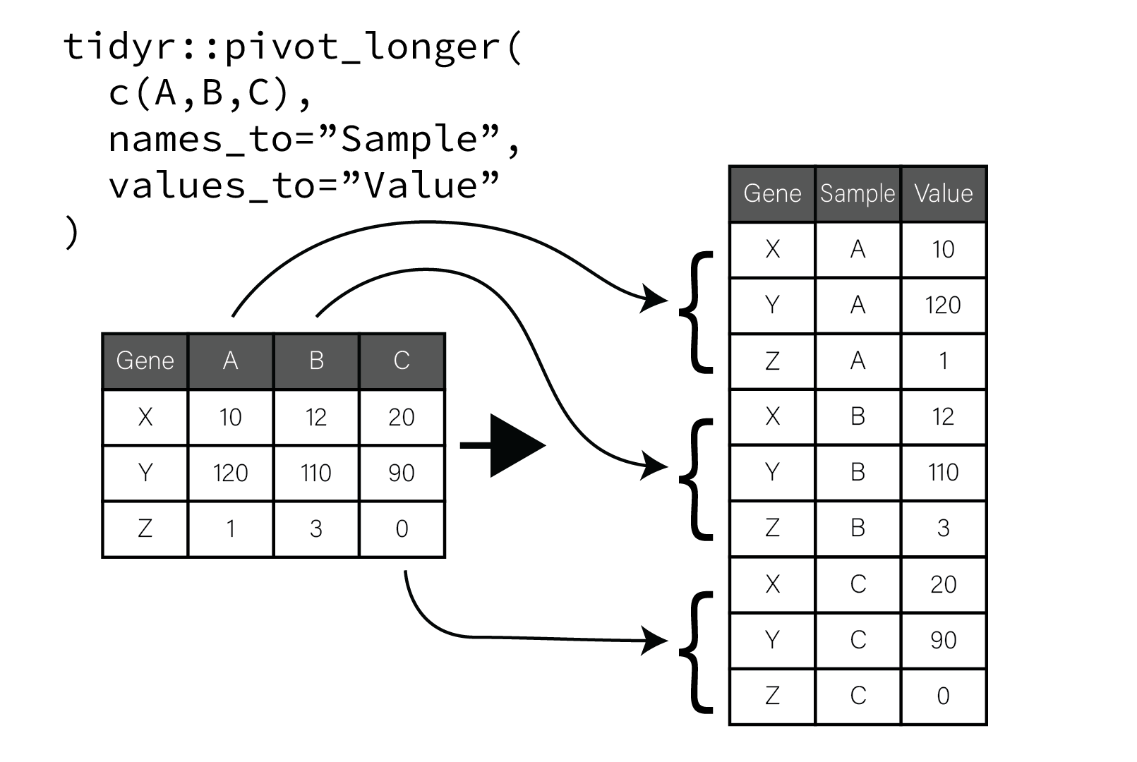
Pivot longer moves columns and values to two new columns

In the figure, the original tibble has genes along rows and samples as columns. When the sample columns are pivoted, the value of each column name is placed in a new column named “Sample” and repeated for as many rows there are in the tibble. A second new column “Value” is populated with the corresponding values that were in each column. The gene associated with each value is preserved and repeated vertically until all the table columns and values have been pivoted. This process of pivoting transforms the tibble into so called “long” form.

Returning to our gene_stats example, we can apply some operations to the tibble to easily perform the summarization we did above in a much more expressive manner:

long_gene_stats <- tidyr::pivot_longer(
  gene_stats,
  ends_with("_stat"),
  names_to="test",
  values_to="stat"
)
long_gene_stats

## # A tibble: 6 × 5
##   gene       test1_p  test2_p test         stat
##   <chr>        <dbl>    <dbl> <chr>       <dbl>
## 1 APOE  0.103        0.000013 test1_stat 12.5  
## 2 APOE  0.103        0.000013 test2_stat 34.2  
## 3 HOXD1 0.632        0.0421   test1_stat  4.40 
## 4 HOXD1 0.632        0.0421   test2_stat 16.3  
## 5 SNCA  0.0000000042 0.915    test1_stat 45.7  
## 6 SNCA  0.0000000042 0.915    test2_stat  0.757

We see that now instead of having X_stat columns, the column names and their values have been put into the test and stat columns, respectively. Now to summarize the statistics for each test, we simply do a group_by() on the test column and compute summaries on the stat column:

long_gene_stats %>%
  dplyr::group_by(test) %>%
  dplyr::summarize(min = min(stat), mean = mean(stat), max = max(stat))

## # A tibble: 2 × 4
##   test         min  mean   max
##   <chr>      <dbl> <dbl> <dbl>
## 1 test1_stat 4.40   20.9  45.7
## 2 test2_stat 0.757  17.1  34.2

You may verify that the numbers are identical in this pivoted tibble as the one we manually created earlier. This pivoting method will produce the desired output regardless of the number of tests we include the table, so long as the column names end in "_test".

The inverse of pivot_longer() is pivot_wider(). If you have variables gathered in single columns like that produced by pivot_longer() you can reverse the process with this function to create a tibble with those variables as columns.

6.10 Relational Data

As mentioned in our section on types of biological data, we often need to combine different sources of data together to aid in interpretation of our results. Below we redefine the tibble of gene statistics from above to have properly capitalized gene symbols:

gene_stats <- tribble(
    ~gene, ~test1_stat, ~test1_p, ~test2_stat, ~test2_p,
   "APOE",   12.509293,   0.1032,   34.239521,   1.3e-5,
  "HOXD1",    4.399211,   0.6323,   16.332318,   0.0421,
   "SNCA",   45.748431,   4.2e-9,    0.757188,   0.9146,
)
gene_stats

## # A tibble: 3 × 5
##   gene  test1_stat      test1_p test2_stat  test2_p
##   <chr>      <dbl>        <dbl>      <dbl>    <dbl>
## 1 APOE       12.5  0.103            34.2   0.000013
## 2 HOXD1       4.40 0.632            16.3   0.0421  
## 3 SNCA       45.7  0.0000000042      0.757 0.915

Our gene identifiers in this data frame are gene symbols which, while convenient for our human brains to remember, can change over time and have many aliases (e.g. the APOE gene has also been called AD2, LDLCQ5, APO-E, and ApoE4 as listed on its genecard). This can make writing code that refers to a specific gene difficult, since there are so many possible names to look for. Fortunately, there are alternative gene identifier systems that do a better job of maintaining stable, consistent gene identifiers, one of the most popular being Ensembl. Ensembl gene IDs always take the form ENSGNNNNNNNNNNN where Ns are digits. These IDs are much more stable and predictable than gene symbols, and are preferable when working with genes in code.

We wish to add Ensembl IDs for the genes in our gene_stats result to the tibble as a new column. Now suppose we have obtained another file with cross referenced gene identifiers like the following:

gene_map <- tribble(
    ~symbol,            ~ENSGID,                    ~gene_name,
     "APOE",  "ENSG00000130203",            "apolipoprotein E",
     "BRCA1",  "ENSG00000012048", "BRCA1 DNA repair associated",
    "HOXD1",  "ENSG00000128645",                 "homeobox D1",
     "SNCA",  "ENSG00000145335",             "synuclein alpha",
)
gene_map

## # A tibble: 4 × 3
##   symbol ENSGID          gene_name                  
##   <chr>  <chr>           <chr>                      
## 1 APOE   ENSG00000130203 apolipoprotein E           
## 2 BRCA1  ENSG00000012048 BRCA1 DNA repair associated
## 3 HOXD1  ENSG00000128645 homeobox D1                
## 4 SNCA   ENSG00000145335 synuclein alpha

Imagine that this file contains mappings for all ~60,000 genes in the human genome. While it might be simple to look up our three genes in this file and annotate manually, it is easier to ask dplyr to do it for us. We can do this using the dplyr::left_join() function which accepts two data frames and the names of columns in each that share common values:

dplyr::left_join(
    x=gene_stats,
    y=gene_map,
    by=c("gene" = "symbol")
)

## # A tibble: 3 × 7
##   gene  test1_stat      test1_p test2_stat  test2_p ENSGID          gene_name   
##   <chr>      <dbl>        <dbl>      <dbl>    <dbl> <chr>           <chr>       
## 1 APOE       12.5  0.103            34.2   0.000013 ENSG00000130203 apolipoprot…
## 2 HOXD1       4.40 0.632            16.3   0.0421   ENSG00000128645 homeobox D1 
## 3 SNCA       45.7  0.0000000042      0.757 0.915    ENSG00000145335 synuclein a…

Notice that the additional columns in gene_map that were not involved in the join (i.e. ENSG and gene_name) are appended to the gene_stats tibble. If we wanted to use pipes, we could implement the same join above as follows:

gene_stats %>% dplyr::left_join(
  gene_map,
  by=c("gene" = "symbol")
)

## # A tibble: 3 × 7
##   gene  test1_stat      test1_p test2_stat  test2_p ENSGID          gene_name   
##   <chr>      <dbl>        <dbl>      <dbl>    <dbl> <chr>           <chr>       
## 1 APOE       12.5  0.103            34.2   0.000013 ENSG00000130203 apolipoprot…
## 2 HOXD1       4.40 0.632            16.3   0.0421   ENSG00000128645 homeobox D1 
## 3 SNCA       45.7  0.0000000042      0.757 0.915    ENSG00000145335 synuclein a…

Under the hood, the dplyr::left_join() function took the values in gene_stats$gene and looked for the corresponding row in gene_map with the same value in in the symbol column. It then appends all the additional columns of gene_map for the matching rows and returns the result. We have added the identifier mapping we desired with only a few lines of code. And what’s more, this code will work no matter how many genes we had in gene_stats as long as gene_map contains a mapping value for the values in gene_stats$gene.

But what happens if we have genes in gene_stats that don’t exist in our mapping? In the above example, we use a left join because we want to include all the rows in gene_stats regardless of whether a mapping exists in gene_map. In this case this was fine because all of our genes in gene_stats had a corresponding row in the mapping. However, notice that in the mapping there is an additional gene, BRCA1 that is not in our gene statistics tibble. If we reverse the order of the join, observe what happens:

gene_map %>% dplyr::left_join(
  gene_stats,
  by=c("symbol" = "gene")
)

## # A tibble: 4 × 7
##   symbol ENSGID          gene_name       test1_stat  test1_p test2_stat  test2_p
##   <chr>  <chr>           <chr>                <dbl>    <dbl>      <dbl>    <dbl>
## 1 APOE   ENSG00000130203 apolipoprotein…      12.5   1.03e-1     34.2    1.3 e-5
## 2 BRCA1  ENSG00000012048 BRCA1 DNA repa…      NA    NA           NA     NA      
## 3 HOXD1  ENSG00000128645 homeobox D1           4.40  6.32e-1     16.3    4.21e-2
## 4 SNCA   ENSG00000145335 synuclein alpha      45.7   4.20e-9      0.757  9.15e-1

Now the order of the rows is the same as in gene_map, and the columns for our missing gene BRCA1 are filled with NA. This is the left join at work, where the record from gene_map is included regardless of whether a corresponding value was found in gene_stats.

There are additional types of joins besides left joins. Right joins are simply the opposite of left joins:

gene_stats %>% dplyr::right_join(
  gene_map,
  by=c("gene" = "symbol")
)

## # A tibble: 4 × 7
##   gene  test1_stat       test1_p test2_stat   test2_p ENSGID          gene_name 
##   <chr>      <dbl>         <dbl>      <dbl>     <dbl> <chr>           <chr>     
## 1 APOE       12.5   0.103            34.2    0.000013 ENSG00000130203 apolipopr…
## 2 HOXD1       4.40  0.632            16.3    0.0421   ENSG00000128645 homeobox …
## 3 SNCA       45.7   0.0000000042      0.757  0.915    ENSG00000145335 synuclein…
## 4 BRCA1      NA    NA                NA     NA        ENSG00000012048 BRCA1 DNA…

The result is the same as the left join on gene_map except the order of the resulting columns is different.

Inner joins return results for rows that have a match between the two tibbles. Recall our left join on gene_map included BRCA1 even though it was not found in gene_stats. An inner join will not include this row, because no match in gene_stats was found:

gene_map %>% dplyr::inner_join(
  gene_stats,
  by=c("symbol" = "gene")
)

## # A tibble: 3 × 7
##   symbol ENSGID          gene_name        test1_stat  test1_p test2_stat test2_p
##   <chr>  <chr>           <chr>                 <dbl>    <dbl>      <dbl>   <dbl>
## 1 APOE   ENSG00000130203 apolipoprotein E      12.5   1.03e-1     34.2   1.3 e-5
## 2 HOXD1  ENSG00000128645 homeobox D1            4.40  6.32e-1     16.3   4.21e-2
## 3 SNCA   ENSG00000145335 synuclein alpha       45.7   4.20e-9      0.757 9.15e-1

One last type of join is the dplyr::full_join() (also sometimes called an outer join). As you may expect, a full join will return all rows from both tibbles whether a match in the other table was found or not.

6.10.1 Dealing with multiple matches

In the example above, there was a one-to-one relationship between the gene symbols in both tibbles. This made the joined tibble tidy. However, when a one-to-many relationship exists, i.e. one gene symbol in one tibble has multiple rows in the other, this can lead to what appears to be duplicate rows in the joined result. Due to the relative instability of gene symbols, it is very common to have multiple Ensembl genes associated with a single gene symbol. The following takes a gene mapping of Ensembl IDs to gene symbols and identifies cases where multiple Ensembl IDs map to a single gene symbol:

readr::read_tsv("mart_export.tsv") %>%
  dplyr::filter(
    `HGNC symbol` != "NA" & # many unstudied genes have Ensembl IDs but no official symbol
    `HGNC symbol` %in% `HGNC symbol`[duplicated(`HGNC symbol`)]) %>%
  dplyr::arrange(`HGNC symbol`)

## # A tibble: 7,268 × 3
##    `Gene stable ID` `HGNC symbol` `Gene name`                                
##    <chr>            <chr>         <chr>                                      
##  1 ENSG00000261846  AADACL2       arylacetamide deacetylase like 2           
##  2 ENSG00000197953  AADACL2       arylacetamide deacetylase like 2           
##  3 ENSG00000262466  AADACL2-AS1   <NA>                                       
##  4 ENSG00000242908  AADACL2-AS1   <NA>                                       
##  5 ENSG00000276072  AATF          apoptosis antagonizing transcription factor
##  6 ENSG00000275700  AATF          apoptosis antagonizing transcription factor
##  7 ENSG00000281173  ABCB10P1      <NA>                                       
##  8 ENSG00000280461  ABCB10P1      <NA>                                       
##  9 ENSG00000274099  ABCB10P1      <NA>                                       
## 10 ENSG00000282479  ABCB10P3      <NA>                                       
## # ℹ 7,258 more rows

There are over 7,000 Ensembl IDs that map to the same gene symbol as another Ensembl ID. That is more than 10% of all Ensembl IDs. So now let’s create a new gene_stats tibble with one of these gene symbols and join with the map to see what happens:

gene_map <- readr::read_tsv("mart_export.tsv")
gene_stats <- tribble(
    ~gene, ~test1_stat, ~test1_p, ~test2_stat, ~test2_p,
   "APOE",   12.509293,   0.1032,   34.239521,   1.3e-5,
  "HOXD1",    4.399211,   0.6323,   16.332318,   0.0421,
   "SNCA",   45.748431,   4.2e-9,    0.757188,   0.9146,
  "DEAF1",    0.000000,      1.0,           0,      1.0
) %>% left_join(gene_map, by=c("gene" = "HGNC symbol"))
gene_stats

## # A tibble: 5 × 7
##   gene  test1_stat      test1_p test2_stat  test2_p `Gene stable ID` `Gene name`
##   <chr>      <dbl>        <dbl>      <dbl>    <dbl> <chr>            <chr>      
## 1 APOE       12.5  0.103            34.2   0.000013 ENSG00000130203  apolipopro…
## 2 HOXD1       4.40 0.632            16.3   0.0421   ENSG00000128645  homeobox D1
## 3 SNCA       45.7  0.0000000042      0.757 0.915    ENSG00000145335  synuclein …
## 4 DEAF1       0    1                 0     1        ENSG00000282712  DEAF1 tran…
## 5 DEAF1       0    1                 0     1        ENSG00000177030  DEAF1 tran…

Notice how there are two rows for the DEAF1 gene that have identical values except for the Stable Gene ID column. This is a very common problem when mapping gene symbols to other gene identifiers and there is no general solution to picking the “best” mapping, short of manually inspecting all of the duplicates and choosing which one is the most appropriate yourself (which obviously is a huge amount of work). However, we do desire to remove the duplicated rows. In this case, since all the values besides the Ensembl ID are the same, effectively it doesn’t matter which duplicate rows we eliminate. We can do this using the duplicated() function, which returns TRUE for all but the first row of a set of duplicated values:

filter(gene_stats, !duplicated(gene))

## # A tibble: 4 × 7
##   gene  test1_stat      test1_p test2_stat  test2_p `Gene stable ID` `Gene name`
##   <chr>      <dbl>        <dbl>      <dbl>    <dbl> <chr>            <chr>      
## 1 APOE       12.5  0.103            34.2   0.000013 ENSG00000130203  apolipopro…
## 2 HOXD1       4.40 0.632            16.3   0.0421   ENSG00000128645  homeobox D1
## 3 SNCA       45.7  0.0000000042      0.757 0.915    ENSG00000145335  synuclein …
## 4 DEAF1       0    1                 0     1        ENSG00000282712  DEAF1 tran…

However, in general, you must be careful about identifying these types of one-to-many mapping issues and also about how you mitigate them.

5 R Programming

7 Data Science