10 EngineeRing

10.1 Unit Testing

Writing code that does what you mean for it to do is often harder than it might seem, especially in R. Also, as your code grows in size and complexity, and you use good programming practice like writing functions, changing one part of your code may have unexpected effects on other parts that you didn’t change. Unless you are using a programming language that has support for proof-based correctness guarantees, it may be impossible to determine if your code is always correct. As you might imagine, so-called “total correctness” is very difficult to attain, and often requires more time to implement than is practical (unless you’re programming something where correctness is very important, e.g. for a self-driving car). However, there is a collection of approaches that can give us reasonable assurances that our code does what we mean for it to do. These approaches are called software testing frameworks that explicitly test our code for correctness.

There are many different testing frameworks, but they all employ the general principle that we test our codes correctness by passing it inputs for which we we know what the output should be. For example, consider the following function that sums two numbers:

add <- function(x,y) {
  return(x+y)
}

We can test this function using a known set of inputs and explicitly comparing the result with the expected output:

result <- add(1,2)
result == 3
[1] TRUE

Our test instance in this case is input x=1,y=2 and the expected output is 3. By comparing the result of this input with the expected output, we have showed that at least for these specific inputs the function behaves as intended. The testing terminology used in this case is the test passed. If the result had been anything other than 3, the test would have failed.

The above is an example of a test, but it is an informal test; it is not yet integrated into a framework since we have to manually inspect the result as passing or failing. In a testing framework, you as the developer of your code also write tests for your code and runs those tests frequently as your code evolves to make sure it continues to behave as you expect over time.

The R package testthat provides such a testing framework that “tries to make testing as fun as possible, so that you get a visceral satisfaction from writing tests.” It’s true that writing tests for your own code may feel tedious and very not fun, but the tradeoff is that tested code is more likely to be correct, saving you from potentially embarrassing (or worse) errors!

Writing tests using testthat is very easy, using the example test written above (remember to install the package using install.packages("testthat") first).

library(testthat)
test_that("add() correctly adds things", {
    expect_equal(add(1,2),3)
    expect_equal(add(5,6),11)
  }
)
Test passed

Test passed! How satisfying! The test_that function accepts two arguments:

1. a concise, human readable description of the test
2. one or more tests enclosed by {} written using expect_X functions from the testthat package

In the example above, we are explicitly testing that the result of add(1,2) is equal to 3 and add(5,6) is equal to 11; specifically, we called expect_equal, which accepts two arguments that it uses to test equality. We have written two explicit test cases (i.e. 1+2 == 3 and 5+6 == 11) under the same test heading.

If we had a mistake in our test such that the expected output was wrong, testthat would inform us not only of the failure, but more details about what happened compared to what we asked it to expect:

test_that("add() correctly adds things", {
    expect_equal(add(1,2),3)
    expect_equal(add(5,6),10)
  }
)
-- Failure (Line 3): add() correctly adds things -------------------------------
add(5, 6) not equal to 10.
1/1 mismatches
[1] 11 - 10 == 1

Error: Test failed

In this case, our test case was incorrect, but this would be very helpful information to have if we had correctly specified input and expected output and the test failed! It means we did something wrong, but now we are aware of it and can fix it.

The general testing strategy usually involves writing an R script that only contains tests like the example above and not analysis code; the tests in your test script call the functions you have written in your other scripts to check for their correctness exactly like above. Then, whenever you make substantial changes to your analysis code, you can simply run your test script to check whether everything went ok. Of course, as you add more functions to your analysis script you need to add new tests for that code. If we had put our test above in a script file called test_functions.R we could run them on our analysis code like the following:

add <- function(x,y) {
return(x+y)
}
testthat::test_file("test_functions.R")

== Testing test_functions.R =======================================================
[ FAIL 0 | WARN 0 | SKIP 0 | PASS 2 ] Done!

The ultimate testing strategy is called test driven development where you write your tests before developing any analysis code, even for functions that don’t exist yet. Imagine we decide we need a new function that multiplies two numbers together and haven’t written it yet. testtthat can handle the situation where you call a function that isn’t defined yet:

test_that("mul() correctly multiplies things",{
expect_equal(mul(1,2),2)
})
-- Error (Line 1): new function ------------------------------------------------
Error in `mul(1, 2)`: could not find function "mul"
Backtrace:
 1. testthat::expect_equal(mul(1, 2), 2)
 2. testthat::quasi_label(enquo(object), label, arg = "object")
 3. rlang::eval_bare(expr, quo_get_env(quo))

Error: Test failed

In this case, the test failed because mul() is not defined yet, but you have already done the hard part of writing the test! Now all you have to do is write the mul() function and keep working on it until the tests pass. Writing tests first and analysis code later is a great way to be thoughtful about how your code is structured, along with the usual benefit of testing that it means your code is more likely to be correct.

• Testing - R packages
• testthat Reference

10.2 Toolification

RStudio is a highly effective tool for developing R code, and most analyses we conduct are suitable for running in its interactive environment. However, there are certain circumstances where running R scripts in this interactive manner is not optimal or even suitable:

1. The same script must be run on many different inputs
2. The data that is to be analyzed is stored on a system where interactive RStudio session are not available
3. The script takes a very long time to run (e.g. days to weeks)
4. The computational demands of the analysis exceed the resources available on the computer where RStudio is being run (e.g. a personal laptop has limited memory)

In these cases, it is necessary to run R scripts outside of RStudio, often on a command line interface (CLI) like that found on linux clusters and cloud based virtual machines. While most scripts can be run in an R interpreter on the CLI and produce the same behavior, there are some steps that help convert an R script into a tool that can be run in this way. This process of transforming an R script in to a more generally usable tool that is run on the CLI is termed toolification in this text. The following sections describe some strategies for toolifying and running R scripts developed in RStudio on the CLI.

10.2.1 The R Interpreter

It bears mentioning that RStudio and R are related but independent programs. Specifically, RStudio runs the R program behind its interface using what is called the R interpreter. When you run R on a CLI, you are given an interactive interface where commands written in the R language can be evaluated. In RStudio, the interpreter that is running behind the scenes can be accessed in the Console tab at the bottom right:

R Interpreter in both RStudio and a linux terminal

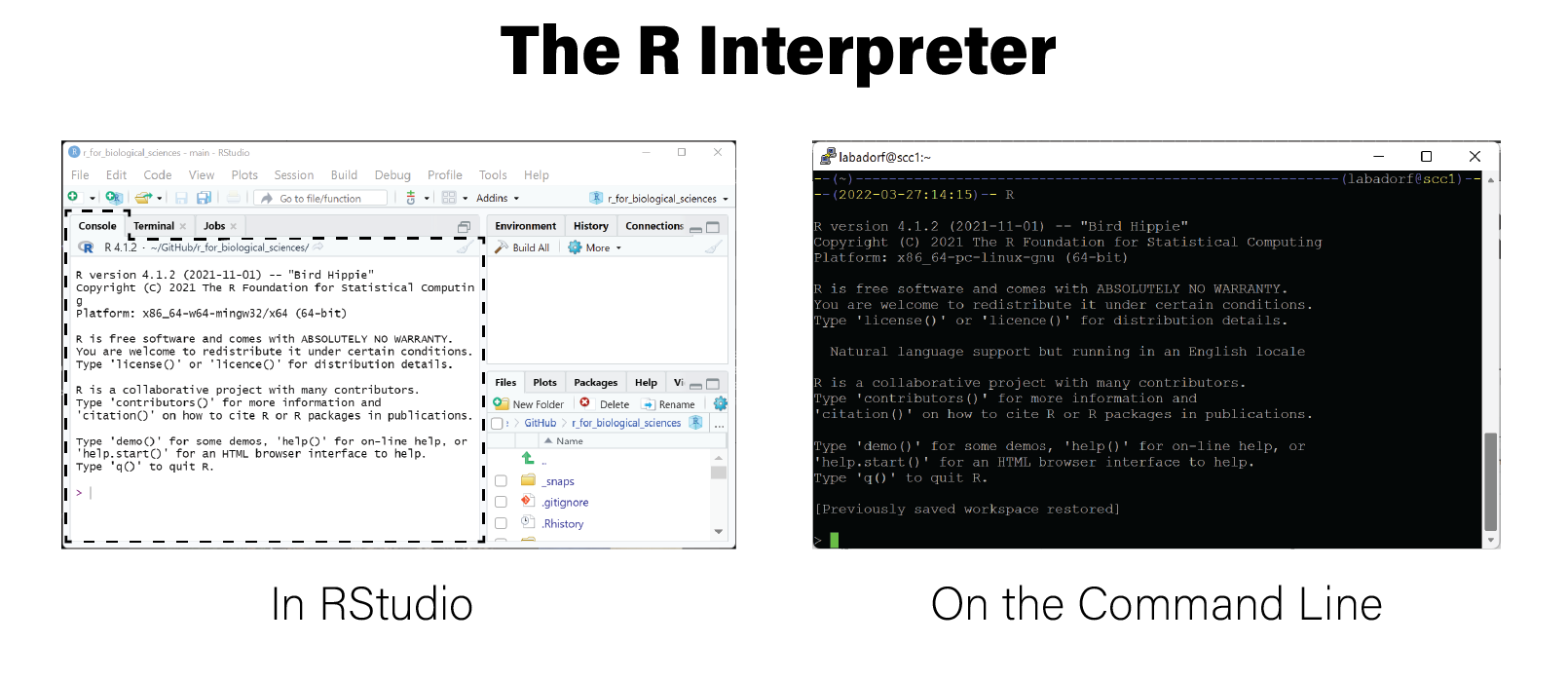
The interpreter by itself is not very useful, since most meaningful analyses require many lines of code be run sequentially as a unit. The interpreter can be helpful to test out individual lines of code and examine help documentation for R functions.

The simplest way to run an R script from the command line is to first run an R interpreter and then use the source() function, which accepts a filename for an R script as its first argument an executes all lines of code in the script.

$ cat simple_script.R
print('hello moon')
print(1+2)
print(str(c(1,2,3,4)))
$ R
> source("simple_script.R")
[1] "hello moon"
[1] 3
 num [1:4] 1 2 3 4

However, this method requires some interactivity, namely by running an R interpreter first, so it is not sufficient to run in a non-interactive fashion. We may need to run our script without any interactivity, for example when it is a part of a computational pipeline.

10.2.2 Rscript

The R program also includes the Rscript command that can be run on the command line:

$ Rscript
Usage: /path/to/Rscript [--options] [-e expr [-e expr2 ...] | file] [args]

--options accepted are
  --help              Print usage and exit
  --version           Print version and exit
  --verbose           Print information on progress
  --default-packages=list
                      Where 'list' is a comma-separated set
                        of package names, or 'NULL'
or options to R, in addition to --no-echo --no-restore, such as
  --save              Do save workspace at the end of the session
  --no-environ        Don't read the site and user environment files
  --no-site-file      Don't read the site-wide Rprofile
  --no-init-file      Don't read the user R profile
  --restore           Do restore previously saved objects at startup
  --vanilla           Combine --no-save, --no-restore, --no-site-file
                        --no-init-file and --no-environ

'file' may contain spaces but not shell metacharacters
Expressions (one or more '-e <expr>') may be used *instead* of 'file'
See also  ?Rscript  from within R

This CLI command accepts an R script as an input and executes the commands in the file as if they had been passed to source(), for example:

$ cat simple_script.R
print('hello moon')
print(1+2)
print(str(c(1,2,3,4)))
$ Rscript simple_script.R
[1] "hello moon"
[1] 3
 num [1:4] 1 2 3 4
$

This is the simplest way to toolify an R script; simply run it on the command line with Rscript. Toolifying simple R scripts that do not need to accept inputs to execute on different data generally require no changes.

Rscript is a convenience function that runs the following R command:

$ Rscript simple_script.R # is equivalent to:
$ R --no-echo --no-restore --file=simple_script.R

If for some reason you cannot run Rscript directly, you can use these arguments with the R command to attain the same result.

10.2.3 commandArgs()

However, sometimes we may wish to control the behavior of a script directly from the command line, rather than editing the script directly for every different execution. To pass information into the script when it is run, we can pass arguments with the Rscript command:

$ Rscript simple_script.R abc
[1] "hello moon"
[1] 3
 num [1:4] 1 2 3 4

Although we passed in the argument abc, the output of the script didn’t change because the script wasn’t written to receive it. In order for a script to gain access to the command line arguments, we must call the commandArgs() function:

args <- commandArgs(trailingOnly=TRUE)

Now when we execute the script, the arguments passed in are available in the args variable:

$ cat echo_args.R
print(commandArgs(trailingOnly=TRUE))
$ Rscript echo_args.R abc
[1] "abc"
$ Rscript echo_args.R abc 123
[1] "abc" "123"
$ Rscript echo_args.R # no args
character(0)

In the last case when no arguments were passed, R is telling us the args variable is a character vector of length zero.

By default, the commandArgs() function will return the full command that was run, including the Rscript command itself and any additional arguments:

$ Rscript -e "commandArgs()" abc 123
[1] "/usr/bin/R"
[2] "--no-echo"
[3] "--no-restore"
[4] "-e"
[5] "commandArgs()"
[6] "--args"
[7] "abc"
[8] "123"

The trailingOnly=TRUE argument returns only the arguments provided at the end of the command, after the Rscript portion:

$ Rscript -e "commandArgs(trailingOnly=TRUE)" abc 123
[1] "abc" "123"

Note you can provide individual commands instead of a script to Rscript with the -e argument.

The commandArgs() function is all that is needed to toolify a R script. Consider a simple script named inspect_csv.R that loads in any CSV file and summarizes it as a tibble:

args <- commandArgs(trailingOnly=TRUE)
if(length(args) != 1) {
  cat("Usage: simple_script.R <csv file>\n") # cat() writes characters to the screen
  cat("Provide exactly one argument that is a CSV filename\n")
  quit(save="no", status=1)
}
fn <- args[1]
library(tidyverse)
read_csv(fn)

We can now run the script with Rscript and give it the filename of a CSV file:

$ cat data.csv
gene,sampleA,sampleB,sampleC
g1,1,35,20
g2,32,56,99
g3,392,583,444
g4,39853,16288,66928
$ Rscript inspect_csv.R data.csv
── Attaching packages ─────────────────────────────────────── tidyverse 1.3.1 ──
✔ ggplot2 3.3.5     ✔ purrr   0.3.4
✔ tibble  3.1.6     ✔ dplyr   1.0.7
✔ tidyr   1.2.0     ✔ stringr 1.4.0
✔ readr   2.1.2     ✔ forcats 0.5.1
── Conflicts ────────────────────────────────────────── tidyverse_conflicts() ──
✖ dplyr::filter() masks stats::filter()
✖ dplyr::lag()    masks stats::lag()
Rows: 4 Columns: 4
── Column specification ────────────────────────────────────────────────────────
Delimiter: ","
chr (1): gene
dbl (3): sampleA, sampleB, sampleC

ℹ Use `spec()` to retrieve the full column specification for this data.
ℹ Specify the column types or set `show_col_types = FALSE` to quiet this message   .
# A tibble: 4 × 4
  gene  sampleA sampleB sampleC
  <chr>   <dbl>   <dbl>   <dbl>
1 g1          1      35      20
2 g2         32      56      99
3 g3        392     583     444
4 g4      39853   16288   66928

Note the input handling of the arguments, where the usage of the script and a helpful error message is printed out before the script quits if there was not exactly one argument provided.

In the example above, a filename was passed into the script as an argument. A filename is encoded as a character string in this case, and commandArgs() always produces a vector of strings. If we need to pass in arguments to control numerical values, we will need to parse the arguments first. Consider the following R implementation of the linux command head, which prints only the top \(n\) lines of a file to the screen:

args <- commandArgs(trailingOnly=TRUE)
if(length(args) != 2) {
      cat("Usage: head.R <filename> <N>\n")
  cat("Provide exactly two arguments: a CSV filename and an integer N\n")
    quit(save="no", status=1)
}

# read in arguments
fn <- args[1]
n <- as.integer(args[2])

# the csv output will include a header row, so reduce n by 1
n <- n-1

# suppressMessages() prevents messages like library loading text from being printed to the screen
suppressMessages(
    {
        library(tidyverse, quietly=TRUE)
        read_csv(fn) %>%
            slice_head(n=n) %>%
            write_csv(stdout())
    }
)

We again tested the number of arguments passed in for correct usage, and then assigned the arguments to variables. The n argument is cast from a character string to an integer in the process, enabling its use in the dplyr::slice_head() function. We can print out the first three lines of a file as follows:

$ Rscript head.R data.csv 3
gene,sampleA,sampleB,sampleC
g1,1,35,20
g2,32,56,99

Reading command line arguments into variables in a script can become tedious if your script has a large number of arguments. Fortunately, the argparser package can help handle many of the repetitive operations, including specifying arguments, providing default values, automatically casting to appropriate types like numbers, and printing out usage information:

library(argparser, quietly=TRUE)
parser <- arg_parser("R implementation of GNU coreutils head command")
parser <- add_argument(parser, "filename", help="file to print lines from")
parser <- add_argument(parser, "-n", help="number of lines to print", type="numeric", default=10)
parser <- parse_args(parser, c("-n",3,"data.csv"))
print(paste("printing from file:",parser$filename))

## [1] "printing from file: data.csv"

print(paste("printing top n:",parser$n))

## [1] "printing top n: 3"

With this library, we can rewrite our head.R script to be more concise:

library(argparser, quietly=TRUE)

# instantiate parser
parser <- arg_parser("R implementation of GNU coreutils head command")

# add arguments
parser <- add_argument(
  parser,
  arg="filename",
  help="file to print lines from"
)
parser <- add_argument(
  parser,
  arg="--top",
  help="number of lines to print",
  type="numeric",
  default=10,
  short='-n'
)

args <- parse_args(parser)

fn <- args$filename

# the csv output will include a header row, so reduce n by 1
n <- args$top-1

suppressMessages(
    {
        library(tidyverse, quietly=TRUE)
        read_csv(fn) %>%
            slice_head(n=n) %>%
            write_csv(stdout())
    }
)

Note we didn’t have to explicitly parse the top argument as an integer because type="numeric" handled this for us. We can print out the top three lines of our file like we did above using the new parser and arguments:

$ Rscript head.R -n 3 data.csv
gene,sampleA,sampleB,sampleC
g1,1,35,20
g2,32,56,99

We can also inspect the usage by passing the -h flag:

$ Rscript head.R -h
usage: head.R [--] [--help] [--opts OPTS] [--top TOP] filename

R implementation of GNU coreutils head command

positional arguments:
  filename    file to print lines from

flags:
  -h, --help  show this help message and exit

optional arguments:
  -x, --opts  RDS file containing argument values
  -n, --top   number of lines to print [default: 10]

These are the only tools required to toolify our R script.

Note that scripts developed in RStudio can be run on the command line, but scripts written for CLI use with the strategies above cannot be easily run inside RStudio! However, if you followed good practices and implemented your script as a set of functions, you can easily write a CLI wapper script that calls those functions, thereby enabling you to continue developing your code in RStudio and maintain CLI tool functionality.

10.3 Parallel Processing

Most modern computers have multiple processing or CPU cores, e.g. a 4-core or 8-core processor. This principally means that these computers can execute multiple processes simultaneously thereby dividing the wall clock time required to run the computations on a one core machine by a factor equal to the number of cores the machine has. This can be a very meaningful performance improvement, e.g. an 8 core machine could reduce the running time of a computation from a week to less than a day. Some data centers possess compute nodes with 28 or even 64 cores, meaning a computation that would normally run for two months could complete in a single day if all cores are used! Processes that are running at the same time on different cores are said to be running in parallel, while a computation that is not parallelized runs serially.

10.3.1 Brief Introduction to Parallelization

Not all computations can be parallelized, and some can only be made parallel by using sophisticated mathematical models and algorithms. However, certain classes of problems are pleasingly parallel, meaning their structure makes it easy if not trivial to divide into parts that can be run in parallel. In general, how “parallelizeable” a computation is depends on how the subparts of the computation relate to one another.

Consider the problem of mapping high throughput sequencing reads against a reference genome. If the task is to identify the location(s) in the genome where each read matches, the locations of one read do not influence the locations of another read; they are independent of each other. Since they are independent, in principle they can be done in parallel, meaning that, again in priniple, every one of the millions of reads could be aligned against the genome at the same time. This would mean the wall clock time required to align all the reads in a multi-million read dataset would take as long as it takes to align a single read. This makes short read alignment a pleasingly parallel problem. Unfortunately, in practice there are technical constraints preventing this increase in performance, but most modern alignment programs like bwa and STAR exploit this inherently parallel structure to improve performance by using multiple cores at the same time.

In general, splitting up a computation into pieces that can run in parallel does not always lead to performance improvements. There are several ways computations are constrained based on which aspects of the algorithm or program require the most time to run. Briefly, an algorithm can be:

• compute-bound - the computations take the largest amount of time
• memory-bound - the amount of main memory (i.e. RAM) on the machine determines how quickly the computation can complete
• input/output (IO)-bound - writing to and from hard disk takes the most time
• network-bound - transfering data over a network, usually between processes running in parallel, takes the most time

These concepts are covered in the field of high-performance computing and are beyond the scope of this class. However, for the purposes of this section, the problems we are concerned with when parallelizing computations are compute-bound computations.

Parallelism can be attained on both the multiprocessor and the distributed computing level. In distributed computing, different subtasks of a parallelizable computation are executed on different physical computers. Each of these subtasks could possibly be further parallelized using multiple cores on each system. In cluster computing or cloud environments, enormous performance improvements can be attained by utilizing both levels of parallelization. For example, if you submit 100 jobs via qsub to a compute cluster and they all run at the same time, and each job uses 16 cores on its local machine, that amounts to a 1,600x speedup. This parallelism would reduce a computation taking over 4 years to run in a single day!

10.3.2 apply and Friends Are Pleasingly Parallel

In R, loops are most efficiently expressed using the apply function and its variants lapply and vapply. Recall that these functions accept a function and a collection of inputs, usually a list. The apply function iterates over the input collection and executes the function on each of them. In general, the inputs are assumed to be independent, and the function does not have any outside dependencies. This is precisely the pattern needed for pleasantly parallel tasks. In general, any iteration using an apply function can be parallelized in R.

10.3.3 The parallel package

R can leverage multiple core architectures to execute processes in parallel with the [parallel package], which is installed as a base R package. The main function in this package that enables parallelism is mclapply(), or multicore apply. mclapply accepts all of the same arguments as lapply and a few additional starting with mc.. The argument to mclapply that enables parallelism is mc.cores, which specifies the number of cores to use when executing tasks in parallel.

mclapply is not available on Windows, only Mac and linux.

Consider the following script mclapply.R which runs a function that prints out its input with the current time and then waits (i.e. sleeps) for three seconds:

library(parallel)

args <- commandArgs(trailingOnly=TRUE)
cores <- as.integer(args[1])

ret <- mclapply(
    1:10,
    function(x) {
         print(paste(Sys.time(),'process',x))
         Sys.sleep(3)
    },
    mc.cores=cores
)

Note the number of cores to be used is passed in as a command line argument. If we run the script with one core, we can see the functions run serially:

$ Rscript mclapply.R 1
[1] "2022-03-23 20:33:09 process 1"
[1] "2022-03-23 20:33:12 process 2"
[1] "2022-03-23 20:33:15 process 3"
[1] "2022-03-23 20:33:18 process 4"
[1] "2022-03-23 20:33:21 process 5"
[1] "2022-03-23 20:33:24 process 6"
[1] "2022-03-23 20:33:27 process 7"
[1] "2022-03-23 20:33:30 process 8"
[1] "2022-03-23 20:33:33 process 9"
[1] "2022-03-23 20:33:36 process 10"

If we instead run the script with three cores, we can see from the printed times that the functions are executed in groups of 3:

$ Rscript mclapply.R 3
[1] "2022-03-23 20:29:56 process 1"
[1] "2022-03-23 20:29:56 process 2"
[1] "2022-03-23 20:29:56 process 3"
[1] "2022-03-23 20:29:59 process 4"
[1] "2022-03-23 20:29:59 process 5"
[1] "2022-03-23 20:29:59 process 6"
[1] "2022-03-23 20:30:02 process 7"
[1] "2022-03-23 20:30:02 process 8"
[1] "2022-03-23 20:30:02 process 9"
[1] "2022-03-23 20:30:05 process 10"

Finally, if we use 10 cores (and the machine we are using has at least 10 cores), all the functions execute simultaneously:

- Rscript mclapply.R 10
[1] "2022-03-23 20:34:59 process 1"
[1] "2022-03-23 20:34:59 process 2"
[1] "2022-03-23 20:34:59 process 3"
[1] "2022-03-23 20:34:59 process 4"
[1] "2022-03-23 20:34:59 process 5"
[1] "2022-03-23 20:34:59 process 6"
[1] "2022-03-23 20:34:59 process 7"
[1] "2022-03-23 20:34:59 process 8"
[1] "2022-03-23 20:34:59 process 9"
[1] "2022-03-23 20:34:59 process 10"

This introduction to parallelization in R will likely be sufficient for most simple parallel tasks, but there are many details that we won’t cover here. For more in-depth explanation of how parallelism in R works refer to the links in the read more box below.

• Parallel Computation section of R Programming for Data Science, by Roger Peng
• Quick Intro to Parallel Computing in R, National Center for Ecological Analysis & Synthesis
• mclapply documentation
• Parallel processing with R on Windows, Water Programming Blog, Reed Lab, Cornell

10.4 Object Oriented Programming in R

Object-orietned programming (OOP) is a programming paradigm that encapsulates related code and data into conceptual “objects”. These objects generally are used to organize code and make it easier to write by passing these encapsulated data and code together as a unit. There are several different styles of OOP, and a programming language my implement more than one style, or none at all.

Although R is primarily a functional programming language it does support OOP in several different ways. Hadley Wickham has written an excellent book chapter on OOP in R and thus is not replicated here.

• OOP in R by Hadley Wickam

10.5 Building R Packages

Packages are the fundamental unit of reproducible code in R. Most of the time, we as practitioners simply use packages that have been provided by others. However, sometimes, when we have developed a methodology that others might find useful, it may be advantageous to write our own R packages and share them with the community. Writing an R package involves creating a directory with a specific structure and adding code, documentation, and package metadata in a way that allows it to be distributed.

Hadley Wickham and Jenny Bryan have written an excellent book on how to write R packages. If ever you need to write your own R package, this should be the only place you need to go.

• R packages by Hadley Wickam and Jenny Bryan