5 R Programming

5.1 Before you begin

If you have not done so already, be sure to follow the R Language, RStudio, and The R Script, and The Scripting Workflow sections before working through this chapter. The guidance in these sections will set you up for success!

5.2 Introduction

As with other subjects covered so far, the basic syntax of R is covered very well in other free online materials. Some of those excellent resources are linked at the end of this section, but a brief overview of the concepts and syntax are covered here. The code examples below can be written into a script and evaluated as described above or entered on the R Console directly and run by pressing Enter.

5.3 R Syntax Basics

At its core, R (like all programming languages) is basically a fancy calculator. The syntax of most basic arithmetic operations in R should be familiar to you:

1 + 2 # addition
[1] 3
3 - 2 # subtraction
[1] 1
4 * 2 # multiplication
[1] 8
4 / 2 # division
[1] 2
1.234 + 2.345 - 3.5*4.9 # numbers can have decimals
[1] -13.571
1.234 + (2.345 - 3.5)*4.9 # expressions can contain parentheses
[1] -4.4255
2**2 # exponentiation
[1] 4
4**(1/2) # square root
[1] 2
9**(1/3) # cube root
[1] 3

The [1] lines above are the output given by R when the preceding expression is executed. Any portion of a line starting with a # is a comment and ignored by R.

R also supports storing values into symbolic placeholders called variables, or objects. An expression like those above can be assigned into a variable with a name using the <- operator:

new_var <- 1 + 2

Variables that have been assigned a value can be placed in subsequent expressions anywhere where their value is evaluated:

new_var - 2
[1] 1
another_var <- new_var * 4

The correct way to assign a value to a variable in R is with the <- syntax, unlike many other programming languages which use =. However, although the = assignment syntax does work in R:

new_var = 2 # works, but is not common convention!

this is considered bad practice and may cause confusion later. You should always use the <- syntax when assigning values to variables!

In R, the period . does not have a special meaning like it does in many other languages like python, C, javascript, etc. Therefore, new.var is a valid variable name just like new_var, even though it may look strange to those familiar with these other languages. While including . in your R variable names is valid, the results that you will use in programs written in other languages that do have a meaning for this character. Therefore, it is good practice to avoid using . characters in your variable names to reduce the chances of conflicts later.

5.4 Basic Types of Values

The most common type of value in R is the number, e.g. 1.0 or 1e-5 for $10^{-5}$. For most practical purposes, R does not distinguish between numbers with fractional parts (e.g. 1.123) and integers (e.g. 1); a number is a number. In addition to numbers, there are some other types of values that are special in R:

logical or boolean values - TRUE or FALSE. Internally, R stores TRUE as the number 1 and FALSE as the number 0. Generally, R interprets non-zero numbers as TRUE and 0 as FALSE, but it is good practice to supply the tokens TRUE or FALSE when an argument expects a logical value.
missing values - NA. NA is a special value that indicates a value is missing.
missing vectors - NULL. Similar to NA, NULL indicates that a vector, rather than a value, is missing. Vectors will be described in the next section on data strutures.
factors - Factors are a complex type used in statistical models and are covered in greater detail later
infinity - Inf and -Inf. These values encode what R understands to be positive or negative infinity, or any number divided by 0.
impossible values - NaN. This value corresponds to the mathematically ‘impossible’ or undefined value of 0/0.
character data - "value". R can store character data in the form of strings. Note R does not interpret string values by default, so "1" and 1 are distinct.
dates and times - R has a basic type to store dates and times (together termed a datetime, which includes both components). Internally, R stores datetimes as the fractional number of days since January 1, 1970, using negative numbers for earlier dates.
complex numbers - R can store complex numbers using the complex function.

Unsurprisingly, R cannot perform computations on NA, NaN, or Inf values. Each of these values have an ‘infectious’ quality to them, where if they are mixed in with other values, the result of the computation reverts to the first of these values encountered:

# this how to create a vector of 4 values in R
x <- c(1,2,3,NA)
mean(x) # compute the mean of values that includes NA
[1] NA
mean(x,na.rm=TRUE) # remove NA values prior to computing mean
[1] 2
mean(c(1,2,3,NaN))
[1] NaN
mean(c(NA,NaN,1))
[1] NA

If your code produces values that are not numbers as you expect, this suggests there are one of these values in your input, and need to be handled explicitly.

5.5 Data Structures

5.5.1 Vectors

Data structures in R (and other languages) are ways of storing and organizing more than one value together. The most basic data structure in R is a one dimensional sequence of values called a vector:

# the c() function creates a vector
x <- c(1,2,3)
[1] 1 2 3

The vector in R has a special property that all values contained in the vector must have the same type, from the list described above. When constructing a vector, R will coerce values to the most general type if it encounters values of different types:

c(1,2,"3")
[1] "1" "2" "3"
c(1,2,TRUE,FALSE)
[1] 1 2 1 0
c(1,2,NA) # note missing values stay missing
[1] 1 2 NA
c("1",2,NA,NaN) # NA stays, NaN is cast to a character type
[1] "1" "2" NA "NaN"

In addition to having a single type, vectors also have a length, which is defined as the number of elements in the vector:

x <- c(1,2,3)
length(x)
[1] 3

Internally, R is much more efficient at operating on vectors than individual elements separately. With numeric vectors, you can perform arithmetic operations on vectors of compatible size just as easily as individual values:

c(1,2) + c(3,4)
[1] 4 6
c(1,2) * c(3,4)
[1] 3 8
c(1,2) * c(3,4,5) # operating on vectors of different lengths raises warning, but still works
[1] 3 8 5
Warning message:
In c(1, 2) * c(3, 4, 5) :
  longer object length is not a multiple of shorter object length

In the example above, we multiplied a vector of length 2 with a vector of length 3:

c(1,2) * c(3,4,5) # operating on vectors of different lengths raises warning, but still works
[1] 3 8 5
Warning message:
In c(1, 2) * c(3, 4, 5) :
  longer object length is not a multiple of shorter object length

Rather than raise an error and aborting, R merely emits a warning message about the vectors not having divisible lengths. So how did R decide the third value should be 5? Because R cycles through each vector and multiplies the values element-wise until the longest vector has had an operation performed on all its values:

c(1,2) * c(3,4,5) # yields: 1*3 2*4 1*5
[1] 3 8 5
Warning message:
In c(1, 2) * c(3, 4, 5) :
  longer object length is not a multiple of shorter object length
c(1,2) * c(3,4,5,6) # yields: 1*3 2*4 1*5 2*6
[1] 3 8 5 12

R will sometimes work in ways you don’t expect. Be careful to read warnings and check that your code does what you expect!

5.5.2 Factors

Factors are objects that R uses to handle categorical variables, i.e. variables that can take one of a distinct set of values for each sample. For example, a variable indicating whether a subject had a disease or was a control could be encoded using a factor with values Disease or Control. Consider an example dataset with six subjects where three are disease and three are control, and we create a factor from a corresponding variable of character strings using the factor() function:

case_status <- factor(
  c('Disease','Disease','Disease',
    'Control','Control','Control'
  )
)
case_status
[1] Disease Disease Disease Control Control Control
Levels: Control Disease

The factor case_status prints as a vector of labels, either Disease or Control. The distinct values in the factor are called levels, and this factor has two: Control and Disease. Internally, a factor is stored as a vector of integers where each level has the same value:

as.numeric(case_status)
[1] 2 2 2 1 1 1
str(case_status)
 Factor w/ 2 levels "Control","Disease": 2 2 2 1 1 1

By default, R assigns integers to levels in alphanumeric order; since “Control” comes lexicographically before “Disease”, the Control level is assigned the integer 1 and Disease is assigned 2. Each value of the factor corresponds to these integers, and since Disease came before Control, the numeric values of the factor are (2, 2, 2, 1, 1, 1). The integer values assigned to each level allow the factor to be sorted:

sort(case_status)
[1] Control Control Control Disease Disease Disease
Levels: Control Disease

Note the order of the factor levels has changed so that controls, which have a value of 1, precede disease, which have a value of 2. The integers assigned to each level can be specified explicitly when creating the factor:

case_status <- factor(
  c('Disease','Disease','Disease','Control','Control','Control'),
  levels=c('Disease','Control')
)
case_status
[1] Disease Disease Disease Control Control Control
Levels: Control Disease
str(case_status)
 Factor w/ 2 levels "Disease","Control": 1 1 1 2 2 2

The base R functions for reading in CSV Files load columns with character values as factors by default (you may turn this off with stringsAsFactors=FALSE to read.csv()), and in other situations you may have factors created by other functions that need to have their integer values changed. This process is called releveling the factor, and may be accomplished by passing a factor into the factor() function and specifying new levels:

str(case_status)
 Factor w/ 2 levels "Disease","Control": 1 1 1 2 2 2
factor(case_status, levels=c("Control","Disease"))
 Factor w/ 2 levels "Control","Disease": 2 2 2 1 1 1

Controlling the order of levels in a factor is important in a number of situations. One is when specifying the reference category for categorical variables when constructing model matrices to pass to statistical models, the details of which are beyond the scope of this book. A second is when the order of categorical variables when passed to ggplot, which is covered in greater detail in [Reordering 1-D Data Elements] in the Grammar of Graphics chapter. The forcats tidyverse package provides more powerful functions for working with categorical variables stored in factors.

5.5.3 Matrices

A matrix in R is simply the 2 dimensional version of a vector. That is, it is a rectangle of values that all have the same type, e.g. number, character, logical, etc. A matrix may be constructed using the vector notation described above and specifying the number of rows and columns the matrix should have, and Instead of having a length like a vector, it has $m \times n$ dimensions:

# create a matrix with two rows and three columns containing integers
A <- matrix(c(1,2,3,4,5,6)
       nrow = 2, ncol = 3, byrow=1
      )
A
[,1] [,2] [,3]
[1,]    1    2    3
[2,]    4    5    6
dim(A) # the dim function prints out the dimensions of the matrix, rows first
[1] 2 3

Because a matrix is 2 dimensional, it can be transposed from $m \times n$ to be $n \times m$ using the t() function:

# A defined above as a 2 x 3 matrix
t(A)
[,1] [,2]
[1,]    1    4
[2,]    2    5
[3,]    3    6
dim(t(A))
[1] 3 2

R can store hyper-rectangular data using arrays. arrays are constructed and operate similarly to matrix, but may have arbitrarily many dimensions. The following example is a 3-dimensional array with dimension sizes of $2x2x3$:

x <- seq(12)
x
[1]  1  2  3  4  5  6  7  8  9 10 11 12
array(x, dim=c(2,2,3))
, , 1

     [,1] [,2]
[1,]    1    3
[2,]    2    4

, , 2

     [,1] [,2]
[1,]    5    7
[2,]    6    8

, , 3

     [,1] [,2]
[1,]    9   11
[2,]   10   12

Hands-On Programming with R - Atomic Vectors R for Data Science - Vectors Advanced R - Vectors

5.5.4 Lists and data frames

Vectors and matrices have the special property that all items must be of the same type, e.g. numbers. Lists and data frames are data structures that do not have this requirement. Similar to vectors, lists and data frames are both one dimensional sequences of values, but the values can be of mixed types. For instance, the first item of a list may be a vector of numbers, while the second is a vector of character strings. These are the most flexible data structures in R, and are among the most commonly used.

Lists can be created using the list() function:

my_list <- list(
  c(1,2,3),
  c("A","B","C","D")
)
my_list
[[1]]
[1] 1 2 3

[[2]]
[1] "A" "B" "C" "D"
my_list[[1]] # access the first item of the list
[1] 1 2 3
my_list[[2]] # access the second item of the list
[1] "A" "B" "C" "D"

The arguments passed to list() define the values and their order of the list. In the above example, the list has two elements: one vector of 3 numbers and one vector of 4 character strings. Note you can access individual items of the list using the [[N]] syntax, where N is the 1-based index of the element.

Lists can also be defined and indexed by name:

my_list <- list(
  numbers=c(1,2,3),
  categories=c("A","B","C","D")
)
my_list
$numbers
[1] 1 2 3

$categories
[1] "A" "B" "C" "D"
my_list$numbers # access the first item of the list
[1] 1 2 3
my_list$categories # access the second item of the list
[1] "A" "B" "C" "D"

The elements of the list have been assigned the names numbers and categories when creating the list, though any valid R identifier names can be used. When elements are associated with names they can be accessed using the list$name syntax.

Lists and data frames are the same underlying data structure, however differ in one important respect: the elements of a data frame must all have the same length, while the elements of a list do not. You may create a data frame with the data.frame() function:

my_df <- data.frame( # recall '.' has no special meaning in R
  numbers=c(1,2,3),
  categories=c("A","B","C","D")
)
Error in data.frame(c(1, 2, 3), c("A", "B", "C", "D")) :
  arguments imply differing number of rows: 3, 4
my_df <- data.frame(
  numbers=c(1,2,3),
  categories=c("A","B","C")
)
my_df
  numbers categories
1       1          A
2       2          B
3       3          C
my_df$numbers
[1] 1 2 3
my_df[1] # numeric indexing also works, and returns a subset data frame
  numbers
1       1
2       2
3       3
my_df[1]$numbers
[1] 1 2 3
# this syntax is [<row>,<column>], and if either is omitted return all
my_df[,1] # return all rows of the first column as a vector
[1] 1 2 3
my_df$categories
[1] "A" "B" "C"

Note the data frame is printed as a matrix with element names as columns and automatically numbered rows. You may access specific elements of a data frame in a number of ways:

my_df$numbers[1] # extract the first value of the numbers column
[1] 1
my_df[1,1] # same as above, recall the [<row>,<column>] syntax
[1] 1
my_df$categories[3] # extract the third value of the categories column
[1] "C"

5.5.5 Subsetting

Each of the data structures in R are collections of objects. Very often, we would like to select a subset of elements in a collection that have certain properties, for instance numeric values less than a specific threshold or occupy a specific position in the vector (e.g. the first or last element). The process of selecting out a subset of elements in a data structure is called subsetting. R provides many different methods to subset a data structure, where the choice of method depends on the type of data structure (e.g. vector vis a vis a data frame) or the type of subsetting required by a particular use case.

Unlike other languages like C and python, R uses 1-based indexing. This means that the first item in any data structure is referenced with the index 1:

x <- c(3.5, 0.4, 9.1, 7.7)
x[1]
[1] 3.5
x[4]
[1] 7.7
x[0] # this always returns an empty vector
[1] numeric(0)
x[5] # accessing indices larger than the vector length returns NA
[1] NA

C and python use 0-based indexing, where the first item in a data structure is referenced with the index 0. For example:

x = [3.5, 0.4, 9.1, 7.7]
print(x[0])
3.5
print(x[3])
7.7
print(x[4]) # accessing indices larger than the list length raises error
Traceback (most recent call last):
  File "<stdin>", line 1, in <module>
IndexError: list index out of range

As you move between developing code in 0-based languages and R, be sure to remember they use different indexing strategies!

5.5.5.1 Vectors

There are six different ways to subset vectors in R. The following three are the most common:

Positive integers: return specific elements by integer index.

x <- c(3.5, 0.4, 9.1, 7.7)
x[1]
[1] 3.5
x[c(1,3)] # can subset using a vector of integers
[1] 3.5 9.1
x[c(1,1)] # can select the same element multiple times
[1] 3.5 3.5

Negative integers: omit specific elements by their negative integer index.

x <- c(3.5, 0.4, 9.1, 7.7)
x[-1] # return all but the first element
[1] 0.4 9.1 7.7
x[-c(2,4)] # return the first and third element
[1] 3.5 9.1

Logical vectors: return specific elements where the indexing vector is TRUE

x <- c(3.5, 0.4, 9.1, 7.7)
x[c(TRUE,FALSE,FALSE,TRUE)]
[1] 3.5
x[c(FALSE,TRUE,TRUE,FALSE)]
[1] 0.4 9.1
x > 3
[1] TRUE FALSE TRUE TRUE
x[x > 3]
[1] 3.5 9.1 7.7

To see the other methods of indexing vectors, see the section on subsetting vectors and Hadley Wickham’s book Advanced R.

5.5.5.2 Matrices

Since matrices in R are vectors, they may be subset using the same methods as vectors. Additionally, because matrices also have a notion of rows and columns, they may also be subset by pairs of vectors that select either rows or columns. A matrix x may be subset with the syntax [<row selectors>, <column selectors>]. The selectors may be any of the methods used to subset a vector, as described above.

x <- matrix(1:9, nrow=3, byrow=TRUE)
x
     [,1] [,2] [,3]
[1,]    1    2    3
[2,]    4    5    6
[3,]    7    8    9
x[c(1,2), c(1,2)] # first two rows, first two columns
     [,1] [,2]
[1,]    1    2
[2,]    4    5
x[-c(1,3), ] # leaving a selector blank selects all, second row and all columns
[1] 4 5 6
x[, c(2,3)] # all rows included, last two columns
     [,1] [,2]
[1,]    2    3
[2,]    5    6
[3,]    8    9
x[-c(1,3), c(2)] # select the second row and second column
[1] 5

5.5.5.3 Lists

A list can be subset with all the same methods as a vector.

l <- list(3.5, 0.4, c(9.1, 5.8), 7.7))
l[1]
[[1]]
[1] 3.5
l[c(2,3)]
[[1]]
[1] 0.4

[[2]]
[1] 9.1 5.8
l[c(FALSE, TRUE, TRUE, FALSE)]
[[1]]
[1] 0.4

[[2]]
[1] 9.1 5.8

Note that when indexing a list with [, the result returned is always another list; we will discuss this more later.

When a list has names associated with its values, it may also be access by name in addition to the ways described above:

l <- list(a=3.5, b=0.4, c=c(9.1, 5.8), d=7.7)
l["a"]
$a
[1] 3.5
l[c("a","c")]
$a
[1] 3.5

$c
[1] 9.1 5.8
l[c("b")]

We will discuss what $ means at the end of this section.

5.5.5.4 Data frames

Data frames may be accessed like both vectors (and therefore lists) and also like matrices, since they are rectangular by construction.

5.5.5.5 `[[` and `$`

The [[ and $ operators are used to access single items of data structures. Remember from the section on subsetting lists that indexing with [ (i.e. a single square bracket) always returns a list. When we wish to access an individual value of a list or data frame and return only that value, we use [[ when indexing by integer or name:

l <- list(a=3.5, b=0.4, c=c(9.1, 5.8), d=7.7)

l[1] # returns a list with a single value of 3.5
[[1]]
[1] 3.5
l[[1]] # returns 3.5
[1] 3.5
l[[3]] # returns c(9.1, 5.8)
[1] 9.1 5.8

l["a"] # returns list(a=3.5)
$a
[1] 3.5
l$a # returns 3.5
[1] 3.5
l[["a"]] # also returns 3.5
[1] 3.5

To see another (ane more complete) treatment of subsetting, see the section on subsetting vectors and Hadley Wickham’s book Advanced R.

Advanced R - Data Structures Advanced R - Subsetting

5.5.6 Naming Data Structures

Vectors, matrices, lists, and data frames can have names assigned to their indices. For vectors and lists, these names are one-dimensional vectors of characters that are assignable and accessible using the names() function:

x <- c(1,2,3)
names(x) # vectors have no names by default
NULL
names(x) <- c("a","b","c")
x
a b c
1 2 3
names(x)
[1] "a" "b" "c"
names(x) <- c("d","e","f")
x
d e f
1 2 3

When a list is created with named items, those names are accessible similarly:

l <- list(a=3.5, b=0.4, c=c(9.1, 5.8), d=7.7)
names(l)
[1] "a" "b" "c" "d"
names(l) <- c("f1", "f2", "f3", "f4")
l
$f1
[1] 3.5

$f2
[1] 0.4

$f3
[1] 9.1 5.8

$f4
[1] 7.7

As matrices and data frames also have both rows and columns, they can have rownames and colnames, respectively:

m <- matrix(1:9, nrow=3, byrow=T)
colnames(m) <- c("c1", "c2", "c3")
rownames(m) <- c("r1", "r2", "r3")
m
   c1 c2 c3
r1  1  2  3
r2  4  5  6
r3  7  8  9
m["r1",] # get row 1
c1 c2 c3 
 1  2  3 
m[, "c2"] # get column 2
r1 r2 r3 
 2  5  8

5.6 Logical Tests and Comparators

As mentioned above, R recognizes logical values as a distinct type. R provides all the conventional infix logical operators:

1 == 1 # equality
[1] TRUE
1 != 1 # inequality
[1] FALSE
1 < 2 # less than
[1] TRUE
1 > 2 # greater than
[1] FALSE
1 <= 2 # less than or equal to
[1] TRUE
1 >= 2 # greater than or equal to

These operators also work on vectors, albeit with the same caveats about vector length as noted earlier:

x <- c(1,2,3)
x == 2
[1] FALSE TRUE FALSE
x < 1
[1] FALSE FALSE FALSE
x < 3
[1] TRUE TRUE FALSE
c(1,2) == c(1,3)
[1] TRUE FALSE
c(1,2) != c(1,3)
[1] FALSE TRUE
c(1,2) == c(1,2,3)
[1] TRUE TRUE FALSE
Warning message:
In c(1, 2, 3) == c(1, 2) :
  longer object length is not a multiple of shorter object length

When performing logical tests on vectors, the all() function may be used to return a single boolean value when all results are true:

x <- c(1,2,3)
all(x == 2)
[1] FALSE
all(x > 0)
[1] TRUE

R also provides many functions of the form is.X where X is some type or condition (recall that . is not a special character in R):

is.numeric(1) # is the argument numeric?
[1] TRUE
is.character(1) # is the argument a string?
[1] FALSE
is.character("ABC")
[1] TRUE
is.numeric(c(1,2,3)) # recall a vector has exactly one type
[1] TRUE
is.numeric(c(1,2,"3"))
[1] FALSE
is.na(c(1,2,NA))
[1] FALSE FALSE TRUE

Quick-R - Operators

5.7 Functions

Just as a variable is a symbolic representation of a value, a function is a symbolic representation of code. In other words, a function allows you to substitute a short name, e.g. mean, for a set of operations on a given input, e.g. the sum of a set of numbers divided by the number of numbers. R provides a very large number of functions for common operations in its default environment, and more functions are provided by packages you can install separately.

Encapsulating many lines of code into a function is useful for (at least) five distinct reasons:

Make your code more concise and readable
Allow you to avoid writing the same code over and over (i.e. reuse it)
Allow you to systematically test pieces of your code to make sure they do what you intend
Allow you to share your code easily with others
Program using a functional programming style (see note box below)

At its core, R is a functional programming language. The details of what this means are outside the scope of this book, but as the name implies this refers to the language being structured around the use of functions. While this property has technical implications on the structure of the language, a more important consequence is the style of programming it entails. The functional programming style (or paradigm) has many advantages, including generally producing programs that are more concise, predictable, provably correct, and performant. provides a good starting point for learning about functional programming.

In order to do anything useful, a function must generally be able to accept and execute on different inputs; e.g. the mean function wouldn’t be very useful if it didn’t accept a value! The terminology used in R and many other programming languages for this is the function must accept or allow you to pass it arguments. In R, functions accept arguments using the following *pattern:

# a basic function signature
function_name(arg1, arg2) # function accepts 2 arguments

Here, arg1 and arg2 are arguments or actual arguments, indicating this function accepts two arguments. The name of the function (i.e. function_name) and the pattern of arguments it accepts is called the function’s signature. Every function has at least one signature, and it is critical to understand it in order to use the function properly.

In the above example, arg1 and arg2 are positional arguments. This means the order of arguments is important. Calling the function above like function_name(arg2, arg1) will produce a different result than with function_name(arg1, arg2). As we will see shortly, functions have names for their arguments in their definition that can be used to specify arguments in any order.

For most functions, some arguments are required. This means that the function will not execute without two arguments provided and will raise an error if you try otherwise:

mean() # compute the arithmetic mean, but of what?
Error in mean.default() : argument "x" is missing, with no default

How do you know what arguments a function requires? All functions provided by base R and many other packages include detailed documentation that can be accessed directly through RStudio using either the ? or help():

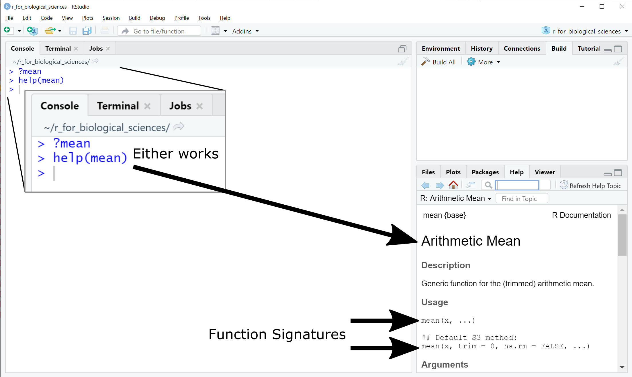
RStudio - help and function signatures

The second signature of the mean function introduces two new types of syntax:

Default argument values - e.g. trim = 0. These are formal arguments that have a default value if not provided explicitly.

Variable arguments - .... This means the mean function can accept arguments that are not explicitly listed in the signature. This syntax is called dynamic dots.

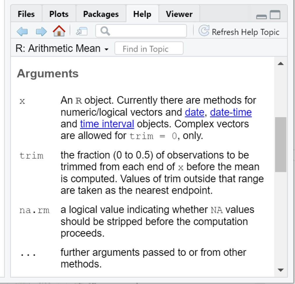
With these definitions, we can now understand the Arguments section of the help documentation:

Arguments to the mean function

In other words:

x is the vector of values (more on this in the next section on data structures) we wish to compute the arithmetic mean for
trim is a fraction (i.e. a number between 0 and 0.5) that instructs R to remove a portion of the largest and smallest values from x prior to computing the mean.
na.rm is a logical value (i.e. either TRUE or FALSE) that instructs R to remove NA values from x before computing the mean.

All function arguments can be specified by name, regardless of whether there is a default value or not. For instance, the following two mean calls are equivalent:

# this generates 100 normally distributed samples with mean 0 and standard deviation 1
my_vals <- rnorm(100,mean=0,sd=1)
mean(my_vals)
[1] -0.05826857
mean(x=my_vals)
[1] -0.05826857

To borrow from the Zen of Python, “Explicit is better than implicit.” Being explicit about which variables are being passed as which arguments will almost always make your code easier to read and more likely to do what you intend.

The ... argument catchall can be very dangerous. It allows you to provide arguments to a function that have no meaning, and R will not raise an error. Consider the following call to mean:

# this generates 100 normally distributed samples with mean 0 and standard deviation 1
my_vals <- rnorm(100,mean=0,sd=1)
mean(x=my_vals,tirm=0.1)
[1] -0.05826857

Did you spot the mistake? The trim argument name has been misspelled as tirm, but R did not report an error. Compare the value of mean without the typo:

mean(x=my_vals,trim=0.1)
[1]-0.02139839

The value we get is different, because R recognizes trim but not tirm and changes its behavior accordingly. Not all functions have the ... catchall in their signatures, but many do and so you must be diligent when supplying arguments to function calls!

5.7.1 DRY: Don’t Repeat Yourself

Sometimes you will find yourself writing the same code more than once to perform the same operation on different data. For example, one common data transformation is standardization or normalization which entails taking a series of numbers, subtracting the mean of all the numbers from them, and dividing each by the standard deviation of the numbers:

# 100 normally distributed samples with mean 20 and standard deviation 10
my_vals <- rnorm(100,mean=20,sd=10)
my_vals_norm <- (my_vals - mean(my_vals))/sd(my_vals)
mean(my_vals_norm)
[1] 0
sd(my_vals_norm)
[1] 1

Later in your code, you may need to standardize a different set of values, so you decide to copy and paste your code from above and replace the variable name to reflect the new data:

# new samples with mean 40 and standard deviation 5
my_other_vals <- rnorm(100,mean=40,sd=5)
my_other_vals_norm <- (my_other_vals - mean(my_other_vals))/sd(my_vals)
mean(my_other_vals_norm)
[1] 0
sd(my_other_vals_norm) # this should be 1!
[1] 0.52351

Notice the mistake? We forgot to change the variable name my_vals to my_other_vals in our pasted code, which produced an incorrect result. Good thing we checked!

In general, if you are copying and pasting code from one part of your script to another, you are repeating yourself and have to do a lot of work to be sure you have modified your copy correctly. Copying and pasting code is tempting from an efficiency standpoint, but introduces may opportunities for (often undetected!) errors.

Don’t Repeat Yourself (DRY) is a principle of software development that emphasizes recognizing and avoiding writing the same code over and over by encapsulating code. In R, this is most easily done with functions. If you notice yourself copying and pasting code, or writing the same pattern of code more than once, this is an excellent opportunity to write your own function and avoid repeating yourself!

5.7.2 Writing your own functions

R allows you to define your own function using the following syntax:

function_name <- function(arg1, arg2, ...) {
  # code that does something with arg1, arg2, etc
  return(some_result)
}

You define the name of your function, the number of arguments it accepts and their names, and the code within the function, which is also called the function body. Taking the example above, I would define a function named standardize that accepts a vector of numbers, subtracts the mean from all the values, and divides them by the standard deviation:

standardize <- function(x) {
  res <- (x - mean(x))/sd(x)
  return(res)
}

my_vals <- rnorm(100,mean=20,sd=10)
my_vals_std <- standardize(my_vals)
mean(my_vals_std)
[1] 0
sd(my_vals_std)
[1] 1

my_other_vals <- rnorm(100,mean=40,sd=5)
my_other_vals_std <- standardize(my_other_vals)
mean(my_other_vals_std)
[1] 0
sd(my_other_vals_std)
[1] 1

Notice above we are assigning the value of the standardize function to new variables. In R and other languages, the result of a function is returned when the function is called; the value returned is called the return value. The return() function makes it clear what the function is returning.

The return() function is not strictly necessary in R; the result of the last line of code in the body of a function is returned by default. However, to again to borrow from the Zen of Python, “Explicit is better than implicit.” Being explicit about what a function returns by using the return() function will make your code less error prone and easier to understand.

5.7.3 Scope

In programming, there is a critically important concept called scope. Every variable and function you define when you program has a scope, which defines where in the rest of your code the variable can be accessed. In R, variables defined outside of a function have universal or top level scope, i.e. they can be accessed from anywhere in your script. However, variables defined inside functions can only be accessed from within that function. For example:

x <- 3
multiply_x_by_two <- function() {
  y <- x*2 # x is not defined as a parameter to the function, but is defined outside the function
  return(y)
}
x
[1] 3
multiply_x_by_two()
[1] 6
y
Error: object 'y' not found

Notice that the variable x is accessible within the function multiply_x_by_two, but the variable y is not accessible outside that function. The reason that x is accessible within the function is that multiply_x_by_two inherits the scope where it is defined, which in this case is the top level scope of your script, which includes x. The scope of y is limited to the body of the function between the { } curly braces defining the function.

Accessing variables within functions from outside the function’s scope is very bad practice! Functions should be as self contained as possible, and any values they need should be passed as parameters. A better way to write the function above would be as follows:

x <- 3
multiply_by_two <- function(x) {
  y <- x*2 # x here is defined as whatever is passed to the function!
  y
}
x
[1] 3
multiply_by_two(6)
[1] 12
x # the value of x in the outer scope remains the same, because the function scope does not modify it
[1] 3

Every variable and function you define is subject to the same scope rules above. Scope is a critical concept to understand when programming, and grasping how it works will make your code more predictable and less error prone.

Scope in R

5.8 Iteration

In programming, iteration refers to stepping sequentially through a set or collection of objects, be it a vector of numbers, the columns of a matrix, etc. In non-functional languages like python, C, etc. there are particular control structures that implement iteration, commonly called loops. If you have worked with these languages, you may be familiar with for and while loops, which are some of these iteration control structures. However, R was designed to execute iteration in a different way than these other languages, and provides two forms of iteration: vectorized operations, and functional programming with apply().

Note that R does have for and while loop support in the language. However, these loop structures can have poor performance, and should generally be avoided in favor of the functional style of iteration described below.

How To Avoid For Loops in R

If you really, really want to learn how to use for loops in R, read this, but don’t say I didn’t warn you when your code slows to a crawl for unknown reasons:

R for Data Science - for loops

5.8.1 Vectorized operations

The simplest form of iteration in R comes in vectorized computation. This sounds fancy, but it just means R intrinsically knows how to perform many operations on vectors and matrices as well as individual values. We have already seen examples of this above when performing arithmetic operations on vectors:

x <- c(1,2,3,4,5)
x + 3 # add 3 to every element of vector x
[1] 4 5 6 7 8
x * x # elementwise multiplication, 1*1 2*2 etc
[1] 1 4 9 16 25
x_mat <- matrix(c(1,2,3,4,5,6),nrow=2,ncol=3)
x_mat + 3 # add 3 to every element of matrix x_mat
[,1] [,2] [,3]
[1,]    4    6    8
[2,]    5    7    9
# the * operator always means element-wise
x_mat * x_mat
     [,1] [,2] [,3]
[1,]    1    9   25
[2,]    4   16   36

In addition to simple arithmetic operations, R also has syntax for vector-vector, matrix-vector, and matrix-matrix operations, like matrix multiplication and dot products:

# the %*% operator stands for matrix multiplication
x_mat %*% c(1,2,3) # [ 2x3 ] * [ 3 ]
     [,1]
[1,]   22
[2,]   28
x_mat %*% t(x_mat) # recall t() is the transpose function, making [ 2x3 ] * [ 3x2 ]
     [,1] [,2]
[1,]   35   44
[2,]   44   56

These forms of implicit iteration are very powerful, and the R program has been highly optimized to perform these operations very quickly. If you can cast your iteration into a vector or matrix multiplication, it is a good idea to do so. For other more complex or custom iteration, we must first talk briefly about functional programming.

5.8.2 Functional programming

R is a functional programming language at its core, which means it is designed around the use of functions. In the previous section, we saw that functions are defined and assigned to names just like variables. This means that functions can be passed to other functions just like variables! Consider the following example.

Let’s consider a general formulation of vector transformation:

\[ \bar{\mathbf{x}} = \frac{\mathbf{x} - t_r(\mathbf{x})}{s(\mathbf{x})} \]

Here, $\mathbf{x}$ is a vector of real numbers, and $\bar{\mathbf{x}}$ is defined as a vector of the same length where each value has had some average or central value $t_r(\mathbf{x})$ subtracted from it, and is divided by a scaling factor $s(\mathbf{x})$ to control the range of resulting values. Both $t_r(\mathbf{x})$ and $s(\mathbf{x})$ are scalars (i.e. individual numbers) and dependent upon the values of $\mathbf{x}$. If $t_r$ is arithmetic mean and $s$ is standard deviation, we have defined the standardization transformation mentioned in earlier examples:

x <- rnorm(100, mean=20, sd=10)
x_zscore <- (x - mean(x))/sd(x)

However, there are many different ways to define the central value of a set of numbers:

arithmetic mean
geometric mean
median
mode
and many more

Each of these central value methods accepts a vector of numbers, but their behaviors are different, and are appropriate in different situations. Likewise, there are many possible scaling strategies we might consider:

standard deviation
rescaling factor (e.g. set data range to be between -1 and 1)
scaling to unit length (all values sum to 1)
and others

We may wish to explore these different methods without writing entirely new code for each combination when trying out different transformation techniques.

In R and other functional languages, we can easily accomplish this by passing functions as arguments to other functions. Consider the following R function:

# note R already has a built in function named "transform"
my_transform <- function(x, t_r, s) {
  return((x - t_r(x))/s(x))
}

This should look familiar to the equation presented earlier, except now in code the arguments t_r and s are passed as arguments. If we wished to transform using a Z-score normalization, we could call my_transform as follows:

x <- rnorm(100,mean=20,sd=10)
x_zscore <- my_transform(x, mean, sd)
mean(x_zscore)
[1] 0
sd(x_zscore)
[1] 1

In the my_transform function call, the second and third arguments are the names of the mean and sd functions, respectively. In the definition of my_transform we use the syntax t_r(x) and s(x) to indicate that these arguments should be treated as functions. Using this strategy, we could just as easily define a transformation using median and sum for t_r and s if we wished to:

x <- rnorm(100,mean=20,sd=10)
x_transform <- my_transform(x, median, sum)
median(x_transform)
[1] 0
sum(x_transform) # this quantity does not have an a priori known value (or meaning for that matter, it's just an example)
[1] 0.013

We can also write our own functions and pass them to get the my_transform function to have desired behavior. The following scales the values of x to have a range of $[0,1]$:

data_range <- function(x) {
  return(max(x) - min(x))
}
# my_transform computes: (x - min(x))/(max(x) - min(x))
x_rescaled <- my_transform(x, min, data_range)
min(x_rescaled)
[1] 0
max(x_rescaled)
[1] 1

The data_range function simply subtracts the minimum value of x from the maximum value and returns the result.

This feature of passing functions as arguments to other functions is a fundamental property of functional programming languages. Now we are ready to finally talk about how iteration is performed in R.

5.8.3 `apply()` and friends

When working with lists and matrices in R, there are often times when you want to perform a computation on every row or every column separately. A common example of this in data science mentioned above is feature standardization. Earlier we wrote a Z-score transformation that accepts a vector, subtracts the mean from each element, and divides the result by the standard deviation of the data. This ensures the data has a mean and standard deviation of 0 and 1, respectively. However, this function only operates on a single vector of numbers. Large datasets have many features, each of which may be individual vectors, that we desire to perform this same Z-score transformation on separately. In other words, we have one function that we wish to execute on either every row or every column of a matrix and return the result. This is a form of iteration that can be implemented in a functional style using the apply function.

This is the signature of the apply function, from the RStudio help(apply) page:

apply(X, MARGIN, FUN, ..., simplify = TRUE)

Here, X is a matrix (i.e. a rectangle of numbers) that we wish to perform a computation on for either each row or each column. MARGIN indicates whether the matrix should be traversed by rows (MARGIN=1) or columns (MARGIN=2). FUN is the name of a function that accepts a vector and returns either a vector or a scalar value that we wish to execute on either the rows or columns. apply() then executes FUN on each row or column of X and returns the result. For example:

zscore <- function(x) {
  return((x-mean(x))/sd(x))
}
# construct a matrix of 50 rows by 100 columns with samples drawn from a normal distribution
x_mat <- matrix(
  rnorm(100*50, mean=20, sd=5),
  nrow=50,
  ncol=100
)
# z-transform the rows of x_mat, so that each column has mean,sd of 0,1
x_mat_zscore  <- apply(x_mat, 2, zscore)
# we can check that all the columns of x_mat_zscore have mean close to zero with apply too
x_mat_zscore_means <- apply(x_mat_zscore, 2, mean)
# note: due to machine precision errors, these results will not be exactly zero, but are very close
# note: the all() function returns true if all of its arguments are TRUE
all(x_mat_zscore_means<1e-15)
[1] TRUE

The same approach can be used when X is a list or data frame rather than a matrix using the lapply() function (hint: the l in lapply stands for “list”). Here is the function signature for lapply:

lapply(X, FUN, ...)

Recall that lists and data frames can be thought of as vectors where each element can be its own vector. Therefore, there is only one axis along which to iterate on the elements and there is not MARGIN argument as in apply. This function returns a new list of the same dimension as the original list with elements returned by FUN:

x <- list(
  feature1=rnorm(100,mean=20,sd=10),
  feature2=rnorm(100,mean=50,sd=5)
)
x_zscore <- lapply(x, zscore)
# check that the means are close to zero
x_zscore_means <- lapply(x_zscore, mean)
all(x_zscore_means < 1e-15)
[1] TRUE

This functional programming pattern might be counter intuitive at first, but it is well worth your while to learn.

R for Data Science - Iteration

5.9 Installing Packages

Advanced functionality in R is provided through packages written and supported by R community members. With the exception of bioconductor packages, all R packages are hosted on the Comprehensive R Archive Network (CRAN) web site. At the time of writing, there are more than 18,000 packages hosted on CRAN that you can install. To install a package from CRAN, use the install.packages function in the R console:

# install one package
install.packages("tidyverse")
# install multiple packages
install.packages(c("readr","dplyr"))

As mentioned above, many packages used in biological data analysis are not hosted on CRAN, but in Bioconductor. The Bioconductor project’s mission is “to develop, support, and disseminate free open source software that facilitates rigorous and reproducible analysis of data from current and emerging biological assays.” Practically, this means Bioconductor packages are subject to stricter standards for documentation, coding conventions and structure, and standards compliance compared with the relatively more lax CRAN package submission process.

5.10 Saving and Loading R Data

While it is always a good idea to save results in tabular form in CSV Files, sometimes it is convenient to save complicated R objects and data structures like lists to a file that can be read back into R easily. This can be done with the saveRDS() and readRDS() functions:

a_complicated_list <- list(
    categories = c("A","B","C"),
    data_matrix = matrix(c(1,2,3,4,5,6),nrows=2,ncols=3),
    nested_list = list(
      a = c(1,2,3),
      b = c(4,5,6)
    )
)
saveRDS(a_complicated_list, "a_complicated_list.rda")

# later, possibly in a different script
a_complicated_list <- readRDS("a_complicated_list.rda")

These functions are very convenient for saving results of complicated analyses and reading them back in later, especially if those analyses were time consuming.

R also has the functions save() and load(). These functions are similar to saveRDS and readRDS, except they do not allow loading individual objects into new variables. Instead, save accepts one or more variable names that are in the global namespace and saves them all to a file:

var_a <- "a string"
var_b <- 1.234

save(var_a, var_b, file="saved_variables.rda")

Then later when the file saved_variables.rda is load()ed, the all the variables saved into the file are loaded into the namespace with their saved values:

# assume var_a and var_b are not defined yet
load("saved_variables.rda")
var_a
[1] "a string"
var_b
[1] 1.234

This requires the programmer to remember the names of the variables that were saved into the file. Also, if there are variables that already exist in the current environment that are also saved in the file, those variable values will be overridden possibly without the programmers knowledge or intent. There is no way to change the variable names of variable saved in this way. For these reasons, saveRDS and loadRDS are generally safer to use as you can be more explicit about what you are saving and loading.

5.11 Troubleshooting and Debugging

Bugs in code are normal. You are not a bad programmer if your code has bugs (thank goodness!). However, some bugs can be very difficult to fix, and some are even difficult to find. You will spend a substantial amount of time debugging your code in R, especially as you are learning the language and its many quirks. You will encounter R error and warning messages routinely during development, and not all of them are straightforward to understand. It is important that you learn how to seek the answers to the problems R reports on your own; your colleagues (and instructors!) will thank you for it.

There is no standard approach to debugging, but here we borrow ideas from Hadley Wickam’s excellent section on debugging in his Advanced R book:

Google! - copy and paste the error into google and see what comes back. Especially when starting out, the errors you receive have been encountered countless times by others before you, and solutions/explanations of them are already out there. If you aren’t already familiar with Stack Overflow, you will be very soon.
Make it repeatable - When you encounter an error, don’t change anything in your code and try again to make sure you get the same error again. This may require you to isolate the code with the error in a different setting to make it more easy to run. If you do, this means the error is repeatable, or replicable, and you can now try modifying the code in question to see if and how the error changes.
Find out where the bug is* - Most bugs involve multiple lines of code, only a subset of which contains the actual error. Sometimes the exact line where the error occurs is obvious, but other times the error is a consequence of a mistake assumption made earlier in the code.
Fix it and test it - When you have identified the specific issue causing the bug, modify the code so it produces the correct result and then rigorously test your fix to make sure it is correct. Sometimes making one change to code causes side effects elsewhere in your code in ways that are difficult to predict. Ideally, you have already written unit tests that explicitly test parts of your code, but if not you will need to use other means of convincing yourself that your fix worked.

This debugging process will become second nature as you work more in R.

Practically speaking, the most basic debugging method is to run code that isn’t working the way it should, print out intermediate results to inspect the state of your variables, and make adjustments accordingly. In RStudio, the Environment Inspector in the top right of the interface makes inspecting the current values of your variables very easy. You can also easily execute lines of code from your script in the interpreter at the bottom right using Cntl-Enter and test out modifications there.

Sometimes you will be working with highly nested data structures like lists of lists. These objects can be difficult to inspect due to their size. The str() function, which stands for structure, will pretty print an object with its values and its structure:

nested_lists <- list(
  a=list(
      item1=c(1,2,3),
      item2=c('A','B','C')
  ),
  b=list(
      var1=1:10,
      var2=100:110,
      var3=1000:1010
  ),  
  c=c(10,9,8,7,6,5)
)
nested_lists
$a
$a$item1
[1] 1 2 3

$a$item2
[1] "A" "B" "C"


$b
$b$var1
 [1]  1  2  3  4  5  6  7  8  9 10

$b$var2
 [1] 100 101 102 103 104 105 106 107 108 109 110

$b$var3
 [1] 1000 1001 1002 1003 1004 1005 1006 1007 1008 1009 1010
str(nested_lists)
List of 3
 $ a:List of 2
  ..$ item1: num [1:3] 1 2 3
  ..$ item2: chr [1:3] "A" "B" "C"
 $ b:List of 3
  ..$ var1: int [1:10] 1 2 3 4 5 6 7 8 9 10
  ..$ var2: int [1:11] 100 101 102 103 104 105 106 107 108 109 ...
  ..$ var3: int [1:11] 1000 1001 1002 1003 1004 1005 1006 1007 1008 1009 ...
 $ c: num [1:6] 10 9 8 7 6 5

The output str is more concise and descriptive than simply printing out the object.

RStudio has many more debugging tools you can use. Check out the section on debugging in Hadley Wickam’s Advanced R book in the Read More box for description of these tools.

Hands-On Programming with R - Debugging R Code Advanced R - Debugging

5.12 Coding Style and Conventions

Some very common worries among new programmers is: “Is my code terrible? How do I write good code?” There is no gold standard for what makes code “good”, but there are some questions you can ask of your code as a guide:

5.12.1 Is my code correct?

Does it produce the desired output? This is pretty obviously important in principle, but it can be difficult to be sure that your code is correct. This is especially difficult if your codebase is large and complicated as it tends to become over time. While simple trial and error is an effective first approach, a more reliable albeit time- and thought-intensive strategy is to write explicit tests for your code and run them regularly.

5.12.2 Does my code follow the DRY principle?

Don’t Repeat Yourself (DRY) is a powerful and helpful strategy to make your code more reliable. This typically involves identifying common patterns in your code and moving them to functions or objects.

5.12.3 Did I choose concise but descriptive variable and function names?

Variable and function names should be descriptive when necessary and not too long. Try to put yourself in the shoes of someone who is reading your code for the first time and see if you can figure out what it does. Better yet, offer to buy a friend a coffee in return for them looking at it!

5.12.4 Did I use indentation and naming conventions consistently throughout my code?

Consistently formatted code is much easier to read (and possibly understand) than inconsistent code. Consider the following code example:

calcVal <- function(x, a, arg=2) { return(sum(x*a)**2)}
calc_val_2 <- function(x, a, b, arg) {
res <- sum(b+a*x)**arg
return(res)}

This code is inconsistent in several ways:

naming conventions - calcVal is camel case, calc_val_2 is snake case
new lines and whitespace - calcVal is all on one line, calc_val_2 is on multiple lines
unhelpful indentation - calc_val_2 has a function body that is not indented, and the close curly brace is appended to the last line of the body
unhelpful function and argument names - the function names describe very little about what the functions do, and the argument names x, a, etc are not very descriptive about what they represent
unused function arguments - the arg argument in calcVal isn’t used anywhere in the function
the two functions appear to do something very similar and could be made simpler using a default argument

A more consistent version of this code might look like:

exponent_product <- function(x, a, offset=0, arg=2) {
  return(sum(offset+a*x)**arg)
}

This code is much cleaner, more consistent, and easier to read.

5.12.5 Did I write comments, especially when what the code does is not obvious?

Sometimes what a piece of code does is obvious from looking at it:

x <- x + 1

Clearly this line of code takes the value of x, whatever it is, and adds 1 to it. However, it may not be obvious why a piece of code does what it does. In these cases, it may be very helpful to record your thinking about a line of code as a comment:

# add 1 as a pseudocount
x <- x + 1

Then when you or someone else reads the code, it will be obvious what you were thinking when you wrote it. In your career, you will encounter situations where you need to figure out what you were thinking when you wrote a piece of code. Endeavor to make future you proud of current you!

5.12.6 How easy would it be for someone else to understand my code?

If someone else who has never seen my code before is asked to run and understand it, how easy would it be for them to do so?

5.12.7 Is my code easy to maintain/change?

This is related to the previous question, but is distinct in that understanding what code does is just the first step in being able to make desired changes to it.

5.12.8 The `styler` package

Consistently formatted code is generally much easier to read than inconsistently formatted code. Consistent formatting may also allow you to identify syntax and logic errors much more easily than it might be otherwise. The styler package is an R package that can automatically format your code to make it consistent in a number of ways, including indentation, code block conventions and more. When you install styler with install.packages("styler") in RStudio, a new entry is available in the Addins menu:

styler Addin menu

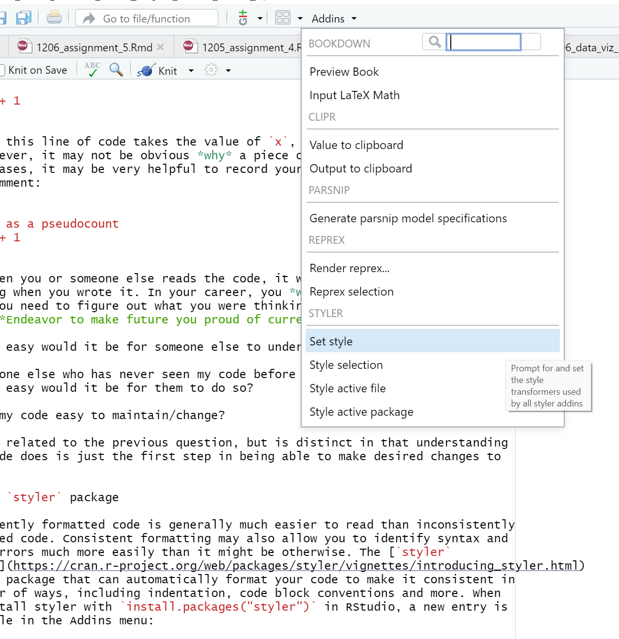
These Addins allow you to let styler format your code for you according to some reasonable (albeit arbitrary) conventions.

4 Preliminaries

6 Data Wrangling