- Syllabus
- 1 Introduction
- 2 Data in Biology
- 3 Preliminaries
- 4 R Programming
- 4.1 Before you begin
- 4.2 Introduction
- 4.3 R Syntax Basics
- 4.4 Basic Types of Values
- 4.5 Data Structures
- 4.6 Logical Tests and Comparators
- 4.7 Functions
- 4.8 Iteration
- 4.9 Installing Packages
- 4.10 Saving and Loading R Data
- 4.11 Troubleshooting and Debugging
- 4.12 Coding Style and Conventions
- 4.12.1 Is my code correct?
- 4.12.2 Does my code follow the DRY principle?
- 4.12.3 Did I choose concise but descriptive variable and function names?
- 4.12.4 Did I use indentation and naming conventions consistently throughout my code?
- 4.12.5 Did I write comments, especially when what the code does is not obvious?
- 4.12.6 How easy would it be for someone else to understand my code?
- 4.12.7 Is my code easy to maintain/change?
- 4.12.8 The
stylerpackage
- 5 Data Wrangling
- 6 Data Science
- 7 Data Visualization
- 8 Biology & Bioinformatics
- 8.1 R in Biology
- 8.2 Biological Data Overview
- 8.3 Bioconductor
- 8.4 Microarrays
- 8.5 High Throughput Sequencing
- 8.6 Gene Identifiers
- 8.7 Gene Expression
- 8.7.1 Gene Expression Data in Bioconductor
- 8.7.2 Differential Expression Analysis
- 8.7.3 Microarray Gene Expression Data
- 8.7.4 Differential Expression: Microarrays (limma)
- 8.7.5 RNASeq
- 8.7.6 RNASeq Gene Expression Data
- 8.7.7 Filtering Counts
- 8.7.8 Count Distributions
- 8.7.9 Differential Expression: RNASeq
- 8.8 Gene Set Enrichment Analysis
- 8.9 Biological Networks .
- 9 EngineeRing
- 10 RShiny
- 11 Communicating with R
- 12 Contribution Guide
- Assignments
- Assignment Format
- Starting an Assignment
- Assignment 1
- Assignment 2
- Assignment 3
- Problem Statement
- Learning Objectives
- Skill List
- Background on Microarrays
- Background on Principal Component Analysis
- Marisa et al. Gene Expression Classification of Colon Cancer into Molecular Subtypes: Characterization, Validation, and Prognostic Value. PLoS Medicine, May 2013. PMID: 23700391
- Scaling data using R
scale() - Proportion of variance explained
- Plotting and visualization of PCA
- Hierarchical Clustering and Heatmaps
- References
- Assignment 4
- Assignment 5
- Problem Statement
- Learning Objectives
- Skill List
- DESeq2 Background
- Generating a counts matrix
- Prefiltering Counts matrix
- Median-of-ratios normalization
- DESeq2 preparation
- O’Meara et al. Transcriptional Reversion of Cardiac Myocyte Fate During Mammalian Cardiac Regeneration. Circ Res. Feb 2015. PMID: 25477501l
- 1. Reading and subsetting the data from verse_counts.tsv and sample_metadata.csv
- 2. Running DESeq2
- 3. Annotating results to construct a labeled volcano plot
- 4. Diagnostic plot of the raw p-values for all genes
- 5. Plotting the LogFoldChanges for differentially expressed genes
- The choice of FDR cutoff depends on cost
- 6. Plotting the normalized counts of differentially expressed genes
- 7. Volcano Plot to visualize differential expression results
- 8. Running fgsea vignette
- 9. Plotting the top ten positive NES and top ten negative NES pathways
- References
- Assignment 6
- Assignment 7
- Appendix
- A Class Outlines
8.7 Gene Expression
Gene expression is the process by which information from a gene is used in the synthesis of functional gene products that affect a phenotype. While gene expression studies are often focused on protein coding genes, there are many other functional molecules, e.g. transfer RNAs, lncRNAs, etc, that are produced by this process. The gene expression process has many steps and intermediate products, as depicted in the following figure:
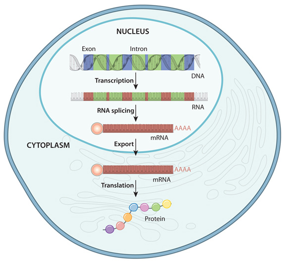
The Gene Expression Process - An overview of the flow of information from DNA to protein in a eukaryote
The specific parts of the genome that code for genes are copied, or transcribed into RNA molecules called transcripts. In lower organisms like bacteria, these RNA molecules are passed on directly to ribosomes, which translate them into proteins. In most higher organisms like eukaryotes, these initial transcripts, called pre-messenger RNA (pre-mRNA) transcripts are further processed such that certain parts of the transcript, called introns, are spliced out and the flanking sequences, called exons, are concatenated together. After this splicing process is complete, the pre-mRNA transcripts become mature messenger RNA (mRNA) transcripts which go on to be exported from the nucleus and loaded into ribosomes in the cytoplasm to undergo translation into proteins.
In gene expression studies, the relative abundance, or number of copies, of RNA or mRNA transcripts in a sample is measured. The measurements are non-negative numbers that are proportional to the relative abundance of a transcript with respect to some reference, either another gene, or in the case of high throughput assays like microarrays or high throughput sequencing, relative to measurements of all distinct transcripts examined in the experiment. Conceptually, the larger the magnitude of a transcript abundance measurement, the more copies of that transcript were in the original sample.
There are many ways to measure the abundance of RNA transcripts; the following are some of the common methods at the time of writing:
- Light absorbance - RNA absorbs ultraviolet light with wavelength 260 nm, which can be used to determine RNA concentration in a sample using specialized equipment
- Northern blot - measures relative abundance of an RNA with a specific sequence
- quantitative polymerase chain reaction (qPCR) - measures relative abundance of an RNA with a specific sequence using PCR amplification
- Oligonucleotide and microarrays - measures relative abundance of thousands of genes simultaneously using known DNA probe sequences and fluorescently tagged RNA molecules
- High throughput RNA sequencing (RNASeq) - measures thousands to millions of RNA fragments simultaneously in proportion to their relative abundance
While any of the measurement methods above may be analyzed in R, the high throughput methods (i.e. microarray, high throughput sequencing) are the primary concern of this chapter. These methods generate measurements for thousands of transcripts or genes simultaneously, requiring the power and flexibility of programmatic analysis to process in a practical amount of time. The remainder of this chapter is devoted to understanding the specific technologies, data types, and analytical strategies involved in working with these data.
Gene expression measurements are almost always inherently relative, either due to limitations of the measurement methods (e.g. microarrays, described below) or because measuring all molecules in a sample will almost always be prohibitively expensive, have diminishing returns, and it is very difficult if not impossible to determine if all the molecules have been measured. This means we cannot in general associate the numbers associated with the measurements with an absolute molecular copy number. An important implication of the inherent relativity of these measurements is: absence of evidence is not evidence of absence. In other words, if a transcript has an abundance measurement of zero, this does not necessarily imply that the gene is not expressed. It may be that the gene is indeed expressed, but the copy number is sufficiently small that it was not detected by the assay.
8.7.1 Gene Expression Data in Bioconductor
The SummarizedExperiment container is the standard way to load and work with gene expression data in Bioconductor. This container requires the following information:
assays- one or more measurement assays (e.g. gene expression) in the form of a feature by sample matrixcolData- metadata associated with the samples (i.e. columns) of the assaysrowData- metadata associated with the features (i.e. rows) of the assaysexptData- additional metadata about the experiment itself, like protocol, project name, etc
The figure below illustrates how the SummarizedExperiment container is structured and how the different data elements are accessed:
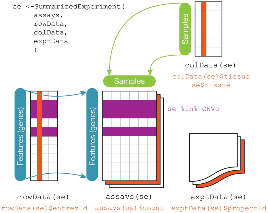
SummarizedExperiment Schematic - Huber, et al. 2015. “Orchestrating High-Throughput Genomic Analysis with Bioconductor.” Nature Methods 12 (2): 115–21.
Many Bioconductor packages for specific types of data, e.g. limma create these SummarizedExperiment objects for you, but you may also create your own by assembling each of these data into data frames manually:
# microarray expression dataset intensities
intensities <- readr::read_delim("example_intensity_data.csv",delim=" ")

# the first column of intensities tibble is the probesetId, extract to pass as rowData
rowData <- intensities["probeset_id"]

# remove probeset IDs from tibble and turn into a R dataframe so that we can assign rownames
# since tibbles don't support row names
intensities <- as.data.frame(
  select(intensities, -probeset_id)
)
rownames(intensities) <- rowData$probeset_id

# these column data are made up, but you would have a sample metadata file to use
colData <- tibble(
  sample_name=colnames(intensities),
  condition=sample(c("case","control"),ncol(intensities),replace=TRUE)
)

se <- SummarizedExperiment(
   assays=list(intensities=intensities),
   colData=colData,
   rowData=rowData
)
se
## class: SummarizedExperiment
## dim: 54675 35
## metadata(0):
## assays(1): intensities
## rownames(54675): 1007_s_at 1053_at ... AFFX-TrpnX-5_at AFFX-TrpnX-M_at
## rowData names(1): probeset_id
## colnames(35): GSM972389 GSM972390 ... GSM972512 GSM972521
## colData names(2): sample_name conditionDetailed documentation of how to create and use the SummarizedExperiment is available in the SummarizedExperiment vignette.
SummarizedExperiment is the successor to the older ExpressionSet container. Both are still used by Bioconductor packages, but SummarizedExperiment is more modern and flexible, so it is suggested for use whenever possible.
8.7.2 Differential Expression Analysis
Differential expression analysis seeks to identify to what extent gene expression is associated with one or more variables of interest. For example, we might be interested in genes that have higher expression in subjects with a disease, or which genes change in response to a treatment.
Typically, gene expression analysis requires two types of data to run: an
expression matrix and a design matrix. The expression matrix will generally
have features (e.g. genes) as rows and samples as columns. The design matrix is
a numeric matrix that contains the variables we wish to model and any covariates
or confounders we wish to adjust for. The variables in the design matrix then
must be encoded in a way that statistical procedures can understand. The full
details of how design matrices are constructed is beyond the scope of this book.
Fortunately, R makes it very easy to construct these matrices from a tibble with
the model.matrix()
function.
Consider for the following imaginary sample information tibble that has 10 AD
and 10 Control subjects with different clinical and protein histology
measurements assayed on their brain tissue:
ad_metadata## # A tibble: 20 x 8
## ID age_at_death condition tau abeta iba1 gfap braak_stage
## <chr> <dbl> <fct> <dbl> <dbl> <dbl> <dbl> <fct>
## 1 A1 81 AD 98543 166078 77299 75277 4
## 2 A2 80 AD 32711 56919 49571 117441 1
## 3 A3 91 AD 134427 295407 106724 67719 6
## 4 A4 90 AD 81515 221801 171212 56346 4
## 5 A5 80 AD 42442 97918 8321 109406 2
## 6 A6 81 AD 54802 49358 82374 42797 2
## 7 A7 77 AD 127166 8417 62675 85377 6
## 8 A8 74 AD 103015 28478 131168 133892 5
## 9 A9 82 AD 114270 188208 194818 61935 5
## 10 A10 83 AD 90785 46279 121555 131853 4
## 11 C1 79 Control 991 237 1062 64752 0
## 12 C2 76 Control 2804 4423 3441 23384 0
## 13 C3 73 Control 3120 7073 1402 135049 0
## 14 C4 73 Control 7167 798 8365 18961 0
## 15 C5 69 Control 6591 2590 4885 65094 0
## 16 C6 77 Control 38697 103664 33430 23136 2
## 17 C7 73 Control 58381 72071 16864 17295 3
## 18 C8 75 Control 5102 10533 5321 89479 0
## 19 C9 76 Control 59906 47967 19103 124651 3
## 20 C10 81 Control 46553 49670 90763 52684 2We might be interested in identifying genes that are increased or decreased in people with AD compared with Controls. We can create a model matrix for this as follows:
model.matrix(~ condition, data=ad_metadata)## (Intercept) conditionAD
## 1 1 1
## 2 1 1
## 3 1 1
## 4 1 1
## 5 1 1
## 6 1 1
## 7 1 1
## 8 1 1
## 9 1 1
## 10 1 1
## 11 1 0
## 12 1 0
## 13 1 0
## 14 1 0
## 15 1 0
## 16 1 0
## 17 1 0
## 18 1 0
## 19 1 0
## 20 1 0
## attr(,"assign")
## [1] 0 1
## attr(,"contrasts")
## attr(,"contrasts")$condition
## [1] "contr.treatment"The ~ condition argument is an an R
forumla,
which is a concise description of how variable should be included in the model.
The general format of a formula is as follows:
# portions in [] are optional
[<outcome variable>] ~ <predictor variable 1> [+ <predictor variable 2>]...

# examples

# model Gene 3 expression as a function of disease status
`Gene 3` ~ condition

# model the amount of tau pathology as a function of abeta pathology,
# adjusting for age at death
tau ~ age_at_death + abeta

# create a model without an outcome variable that can be used to create the
# model matrix to test for differences with disease status adjusting for age at death
~ age_at_death + condition
For most models, the design matrix will have an intercept term of all ones and
additional colums for the other variables in the model. We might wish to adjust
out the effect of age by including age_at_death as a covariate in the model:
model.matrix(~ age_at_death + condition, data=ad_metadata)## (Intercept) age_at_death conditionAD
## 1 1 81 1
## 2 1 80 1
## 3 1 91 1
## 4 1 90 1
## 5 1 80 1
## 6 1 81 1
## 7 1 77 1
## 8 1 74 1
## 9 1 82 1
## 10 1 83 1
## 11 1 79 0
## 12 1 76 0
## 13 1 73 0
## 14 1 73 0
## 15 1 69 0
## 16 1 77 0
## 17 1 73 0
## 18 1 75 0
## 19 1 76 0
## 20 1 81 0
## attr(,"assign")
## [1] 0 1 2
## attr(,"contrasts")
## attr(,"contrasts")$condition
## [1] "contr.treatment"The model matrix now includes a column for age at death as well. This model model matrix is now suitable to pass to differential expression software packages to look for genes associated with disease status.
As mentioned above, modern gene expression assays measure thousands of genes simultaneously. This means each gene must be tested for differential expression individually. In general, each gene is tested using the same statistical model, so a differential expression analysis package will perform something equivalent to the following:
Gene 1 ~ age_at_death + condition
Gene 2 ~ age_at_death + condition
Gene 3 ~ age_at_death + condition
...
Gene N ~ age_at_death + condition
Each gene model will have its own statistics associated with it that we must process and interpret after the analysis is complete.
8.7.3 Microarray Gene Expression Data
On a high level, there are four steps involved in analyzing gene expression microarray data:
- Summarization of probes to probesets. Each gene is represented by multiple probes with different sequences. Summarization is a statistical procedure that computes a single value for each probeset from its corresponding probes.
- Normalization. This includes removing background signal from individual arrays as well as adjusting probeset intensities so that they are comparable across multiple sample arrays.
- Quality control. Compare all normalized samples within a sample set to identify, mitigate, or eliminate potential outlier samples.
- Analysis. Using the quality controlled expression data, Implement statistical analysis to answer research questions.
The full details of microarray analysis are beyond the scope of this book. However in the following sections we cover some of the basic entry points to performing these steps in R and Bioconductor.
The CEL data files from a set of microarrays can be loaded into R for analysis
using the affy Bioconductor
package.
This package provides all the functions necessary for loading the data and
performing key preprocessing operations. Typically, two or more samples were
processed in this way, resulting in a set of CEL files that should be processed
together. These CEL files will typically be all stored in the same directory,
and may be loaded using the affy::ReadAffy function:
# read all CEL files in a single directory
affy_batch <- affy::ReadAffy(celfile.path="directory/of/CELfiles")

# or individual files in different directories
cel_filenames <- c(
  list.files( path="CELfile_dir1", full.names=TRUE, pattern=".CEL$" ),
  list.files( path="CELfile_dir2", full.names=TRUE, pattern=".CEL$" )
)
affy_batch <- affy::ReadAffy(filenames=cel_filenames)
The affy_batch variable is a AffyBatch container, which stores information
on the probe definitions based on the type of microarray, probe-level intensity
for each sample, and other information about the experiment contained within the
CEL files.
The affy package provides functions to perform probe summarization and
normalization. The most popular method to accomplish this at the time of writing
is called Robust Multi-array Average or RMA (Irizarry et al. 2003), which performs
summarization and normalization of multiple arrays simultaneously. Below, the
RMA algorithm is used to normalize an example dataset provided by the
affydata
Bioconductor package.
Certain Bioconductor packages provide example datasets for use with companion
analysis packages. For example, the affydata package provides the Dilution
dataset, which was generated using two concentrations of cDNA from human liver
tissue and a central nervous system cell line. To load a data package into R,
first run library(<data package>) and then data(<dataset name>).
library(affy)
library(affydata)
## Package LibPath Item
## [1,] "affydata" "C:/Users/Adam/Documents/R/win-library/4.1" "Dilution"
## Title
## [1,] "AffyBatch instance Dilution"data(Dilution)
# normalize the Dilution microarray expression values
# note Dilution is an AffyBatch object
eset_rma <- affy::rma(Dilution,verbose=FALSE)
# plot distribution of non-normalized probes
# note rma normalization takes the log2 of the expression values,
# so we must do so on the raw data to compare
raw_intensity <- as_tibble(exprs(Dilution)) %>%
mutate(probeset_id=rownames(exprs(Dilution))) %>%
pivot_longer(-probeset_id, names_to="Sample", values_to = "Intensity") %>%
mutate(
`log2 Intensity`=log2(Intensity),
Category="Before Normalization"
)
# plot distribution of normalized probes
rma_intensity <- as_tibble(exprs(eset_rma)) %>%
mutate(probesetid=featureNames(eset_rma)) %>%
pivot_longer(-probesetid, names_to="Sample", values_to = "log2 Intensity") %>%
mutate(Category="RMA Normalized")
dplyr::bind_rows(raw_intensity, rma_intensity) %>%
ggplot(aes(x=Sample, y=`log2 Intensity`)) +
geom_boxplot() +
facet_wrap(vars(Category))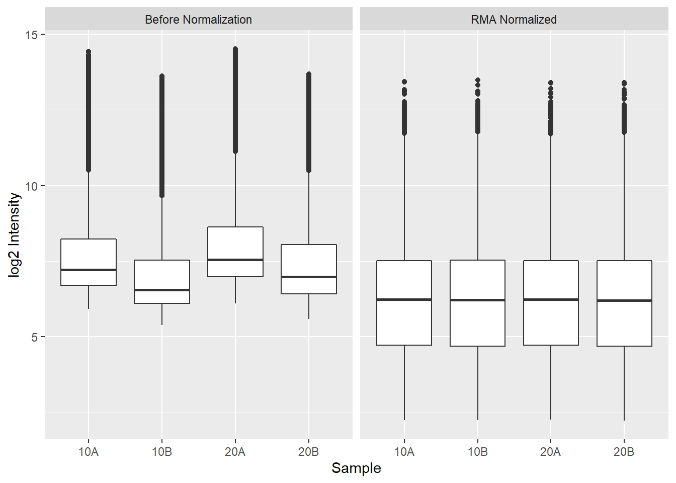
Above, we first apply RMA to the Dilution microarray dataset using the
affy::rma() function. Then we plot the log 2 intensities of the probes in each
array, first using the raw intensities and then afysis seeking to
identify how associated gene expression is with one or more variables of
interest. For example,
8.7.4 Differential Expression: Microarrays (limma)
limma, which
is short for linear models of microarrays, is one of the top most
downloaded Bioconductor packages.
limma is utilized for analyzing microarray gene expression data, with a focus on
analyses using linear models to integrate all of the data from an experiment.
limma was developed for microarray analysis prior to the development of
sequencing based gene expression methods (i.e. RNASeq) but has since added
functionality to analyze other types of gene expression data.
limma excels at analyzing these types of data as it can support arbitrarily complex experimental designs while maintaining strong statistical power. An experiment with a large number of conditions or predictors can still be analyze even with small sample sizes. The method accomplishes this by using an empirical Bayes approach that borrows information across all the genes in the dataset to better control error in individual gene models. See Ritchie et al. (2015) for more details on how limma works.
limma requres an expression matrix like that stored in an ExpressionSet or SummarizedExperiment container and a design matrix:
# intensities is an example gene expression matrix that corresponds to our
# AD sample metadata of 10 AD and 10 Control individuals
ad_se  <- SummarizedExperiment(
  assays=list(intensities=intensities),
  colData=ad_metadata,
  rowData=rownames(intensities)
)

# define our design matrix for AD vs control, adjusting for age at death
ad_vs_control_model <- model.matrix(~ age_at_death + condition, data=ad_metadata)

# now run limma
# first fit all genes with the model
fit <- limma::lmFit(
  assays(se)$intensities,
  ad_vs_control_model
)

# now better control fit errors with the empirical Bayes method
fit <- limma::eBayes(fit)
We have now conducted a differential expression analysis with limma. We can
extract out the results for our question of interest - which genes are
associated with AD - using the limma::topTable() function:
# the coefficient name conditionAD is the column name in the design matrix
# adjust="BH" means perform Benjamini-Hochberg multiple testing adjustment
# on the nominal p-values from each gene test
# topTable only returns the top 10 results sorted by ascending p-value by default
topTable(fit, coef="conditionAD", adjust="BH")
## logFC AveExpr t P.Value adj.P.Val B
## 234942_s_at 1.1231942 8.397425 4.890779 9.613196e-05 0.770605 -2.987573
## 202423_at -0.7499088 8.646687 -4.785281 1.221646e-04 0.770605 -3.025525
## 1557538_at -0.8057310 4.348859 -4.697520 1.492072e-04 0.770605 -3.057737
## 1558290_a_at -0.8580750 7.278878 -4.658725 1.630238e-04 0.770605 -3.072162
## 234596_at 0.4925167 3.038448 4.564888 2.020432e-04 0.770605 -3.107523
## 225986_x_at -0.6030385 6.958092 -4.502976 2.328354e-04 0.770605 -3.131216
## 203124_s_at -1.2857166 8.565022 -4.488589 2.406451e-04 0.770605 -3.136763
## 209346_s_at 0.6578475 6.010219 4.421869 2.804637e-04 0.770605 -3.162688
## 224825_at 1.0266849 8.147104 4.421597 2.806391e-04 0.770605 -3.162795
## 205647_at -0.8569475 4.399029 -4.399700 2.951151e-04 0.770605 -3.171376From the table, none of the probesets in this experiment are significant at FDR < 0.05.
8.7.5 RNASeq
RNA sequencing (RNASeq) is a HTS technology that measures the abundance of RNA molecules in a sample. Briefly, RNA molecules are extracted from a sample using a biochemical protocol that isolates RNA from other molecules (i.e. DNA, proteins, etc) in the sample. Ribosomal RNA is removed from the sample (see Note box below), and the remaining RNA molecules are size selected to retain only short molecules (~15-300 nucleotides in length, depending on the protocol). The size selected molecules are then reverse transcribed into cDNA and converted to double stranded molecules. Sequencing libraries are prepared with these cDNA using proprietary biochemical protocols to make them suitable for sequencing on the sequencing instrument. After sequencing, FASTQ files containing millions of reads for one or more samples is produced. Except for the initial RNA extraction, all of these steps are typically performed by specialized instrumentation facilities called sequencing cores who provide the data in FASTQ format to the investigators.
80%-90% of the RNA mass in a cell is ribosomal RNA (rRNA), the RNA that makes up ribosomes and is responsible for maintaining protein translation processes in the cell. If total RNA was sequenced, the large majority of reads would correspond to rRNAs and would therefore be of little or no use. For this reason, rRNA molecules are removed from the RNA material that goes on to sequencing using either a poly-A tail enrichment or ribo-depletion strategy. These two methods maintain different populations of RNA and therefore sequencing datasets generated with different strategies require different interpretations. The more detail on this topic is beyond the scope of this book, but (Zhao et al. 2018) provide a good introduction and comparison of both approaches.
The reads produced in an RNASeq experiment represent RNA fragments from transcripts. The number of reads that correspond to specific transcripts is assumed to be proportional to the copy number of that transcript in the original sample. The alignment process described in the Preliminary HTS Data Analysis section produces alignments of reads against the genome or transcriptome, and the number of reads that align against each gene or transcript is counted using a reference annotation that defines the locations of every known gene in the genome. The resulting counts are therefore estimates of the copy number of the molecules for each gene or transcript in the original sample. Conceptually, the more reads that map to a gene, the higher the abundance of transcripts for that gene, and therefore we infer higher the expression of that gene.
Gene expression for different genes can vary by orders of magnitude within a single cell, where highly expressed genes may have billions of transcripts and others comparatively few. Therefore, the likelihood of obtaining a read for a given transcript is proportional to the relative abundance of that transcript compared with all other transcripts. Relatively rare transcripts have a low probability of being sampled by the sequencing procedure, and extremely lowly expressed genes may not be sampled at all. The library size (i.e. the total number of reads) in the sequencing dataset for a sample determines the range of gene expression the dataset is likely to detect, where datasets with few reads are unlikely to sample lowly expressed transcripts even though they are truly expressed. For this reason absence of evidence is not evidence of absence in RNASeq data. If a read is not observed for any given gene, we cannot say that the gene is not expressed; we can only say that the relative expression of that gene is below the detection threshold of the dataset we generated, given the number of sequenced reads.
For a single sample, the output of this read counting procedure is a vector of read counts for each gene in the annotation. Genes with no reads mapping to them will have a count of zero, and all others will have a read count of one or more; as mentioned in the Count Data section, read counts are typically non-zero integers. This procedure is typically repeated separately for a set of samples that make up the experiment, and the counts for each sample are concatenated together into a counts matrix. This count matrix is the primary result of interest that is passed on to downstream analysis, most commonly differential expression analysis.
8.7.6 RNASeq Gene Expression Data
The read counts for each gene or transcript in the genome are estimates of the relative abundance of molecules in the original sample. The number of genes counted depends on the organism being studied and the maturity of the gene annotation used. Complex multicellular organisms have on the order of thousands to tens of thousands of genes; for example, humans and mice have 20k-30k genes in their respective genomes. Each RNASeq experiment thus may yield tens of thousands of measurements for each sample.
We shall consider an example RNASeq dataset generated by (O’Meara et al. 2015) generated to study how mouse cardiac cells can regenerate up until one week of age, after which they lose the ability to do so. The dataset has eight RNASeq samples, two for each of four time points across the developmental window until adulthood. We will load in the expression data as a tibble:
counts <- read_tsv("verse_counts.tsv")
counts
## # A tibble: 55,416 x 9
## gene P0_1 P0_2 P4_1 P4_2 P7_1 P7_2 Ad_1 Ad_2
## <chr> <dbl> <dbl> <dbl> <dbl> <dbl> <dbl> <dbl> <dbl>
## 1 ENSMUSG00000102693.2 0 0 0 0 0 0 0 0
## 2 ENSMUSG00000064842.3 0 0 0 0 0 0 0 0
## 3 ENSMUSG00000051951.6 19 24 17 17 17 12 7 5
## 4 ENSMUSG00000102851.2 0 0 0 0 1 0 0 0
## 5 ENSMUSG00000103377.2 1 0 0 1 0 1 1 0
## 6 ENSMUSG00000104017.2 0 3 0 0 0 1 0 0
## 7 ENSMUSG00000103025.2 0 0 0 0 0 0 0 0
## 8 ENSMUSG00000089699.2 0 0 0 0 0 0 0 0
## 9 ENSMUSG00000103201.2 0 0 0 0 0 0 0 1
## 10 ENSMUSG00000103147.2 0 0 0 0 0 0 0 0
## # ... with 55,406 more rowsThe annotation counted reads for 55,416 annnotated Ensembl gene for the mouse genome, as described in the Gene Identifier Systems section.
There are typically three steps when analyzing a RNASeq count matrix:
- Filter genes that are unlikely to be differentially expressed.
- Normalize filtered counts to make samples comparable to one another.
- Differential expression analysis of filtered, normalized counts.
Each of these steps will be described in detail below.
8.7.7 Filtering Counts
Filtering genes that are not likely to be differentially expressed is an important step in differential expression analysis. The primary reason for this is to reduce the number of genes tested for differential expression, thereby reducing the multiple testing burden on the results. There are many approaches and rationales for picking filters, and the choice is generally subjective and highly dependent upon the specific dataset. In this section we discuss some of the rationale and considerations for different filtering strategies.
Genes that were not detected in any sample are the easiest to filter, and often eliminate many genes from consideration. Below we filter out all genes that have zero counts in all samples:
nonzero_genes <- rowSums(counts[-1])!=0
filtered_counts <- counts[nonzero_genes,]
filtered_counts
## # A tibble: 32,613 x 9
## gene P0_1 P0_2 P4_1 P4_2 P7_1 P7_2 Ad_1 Ad_2
## <chr> <dbl> <dbl> <dbl> <dbl> <dbl> <dbl> <dbl> <dbl>
## 1 ENSMUSG00000051951.6 19 24 17 17 17 12 7 5
## 2 ENSMUSG00000102851.2 0 0 0 0 1 0 0 0
## 3 ENSMUSG00000103377.2 1 0 0 1 0 1 1 0
## 4 ENSMUSG00000104017.2 0 3 0 0 0 1 0 0
## 5 ENSMUSG00000103201.2 0 0 0 0 0 0 0 1
## 6 ENSMUSG00000103161.2 0 0 1 0 0 0 0 0
## 7 ENSMUSG00000102331.2 5 8 2 6 6 11 4 3
## 8 ENSMUSG00000102343.2 0 0 0 1 0 0 0 0
## 9 ENSMUSG00000025900.14 4 3 6 7 7 3 36 35
## 10 ENSMUSG00000102948.2 1 0 0 0 0 0 0 1
## # ... with 32,603 more rowsOnly 32,613 genes remain after filtering out genes with all zeros, eliminating nearly 23,000 genes, or more than 40% of the genes in the annotation. Filtering genes with zeros in all samples as we have done above is somewhat liberal, as there may be many genes with reads in only one sample. Genes with only a single sample with a non-zero count also cannot be differentially expressed, so we can easily decide to eliminate those as well:
nonzero_genes <- rowSums(counts[-1])>=2
filtered_counts <- counts[nonzero_genes,]
filtered_counts
## # A tibble: 28,979 x 9
## gene P0_1 P0_2 P4_1 P4_2 P7_1 P7_2 Ad_1 Ad_2
## <chr> <dbl> <dbl> <dbl> <dbl> <dbl> <dbl> <dbl> <dbl>
## 1 ENSMUSG00000051951.6 19 24 17 17 17 12 7 5
## 2 ENSMUSG00000103377.2 1 0 0 1 0 1 1 0
## 3 ENSMUSG00000104017.2 0 3 0 0 0 1 0 0
## 4 ENSMUSG00000102331.2 5 8 2 6 6 11 4 3
## 5 ENSMUSG00000025900.14 4 3 6 7 7 3 36 35
## 6 ENSMUSG00000102948.2 1 0 0 0 0 0 0 1
## 7 ENSMUSG00000025902.14 195 186 204 229 157 173 196 129
## 8 ENSMUSG00000104238.2 0 4 0 2 4 1 3 3
## 9 ENSMUSG00000102269.2 7 16 6 6 4 6 8 3
## 10 ENSMUSG00000118917.1 0 1 0 0 1 1 0 0
## # ... with 28,969 more rowsWe have now reduced our number of genes to 28,979 by including only genes with at least two non-zero counts. We may now wonder how many genes we would include if we required at least \(n\) samples to have non-zero counts. Consider the following bar chart of the number of genes detected in at least \(n\) samples:
library(patchwork)

nonzero_counts <- mutate(counts,`Number of samples`=rowSums(counts[-1]!=0)) %>%
  group_by(`Number of samples`) %>%
  summarize(`Number of genes`=n() ) %>%
  mutate(`Cumulative number of genes`=sum(`Number of genes`)-lag(cumsum(`Number of genes`),1,default=0))

sum_g <- ggplot(nonzero_counts) +
  geom_bar(aes(x=`Number of samples`,y=`Cumulative number of genes`,fill="In at least n"),stat="identity") +
  geom_bar(aes(x=`Number of samples`,y=`Number of genes`,fill="In exactly n"),stat="identity") +
  labs(title="Number of genes detected in n samples") +
  scale_fill_discrete(name="Nonzero in:")

sum_g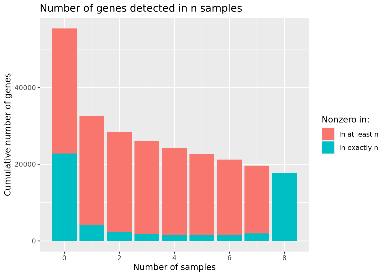
The largest number of genes is detected in none of the samples, followed by genes detected in all samples, with many fewer in between. Based on the plot, there is no obvious choice for how many nonzero samples are sufficient to use as a filter.
We may gain additional insight into this problem by considering the distribution of counts for genes present in at least \(n\) samples as above, rather than just the number of nonzero counts. Below is a plot similar to that above but, which plots the distribution of mean counts across samples within each number of nonzero samples:
# calculate the mean count for non-zero counts in genes with exactly n non-zero counts
mutate(counts,`Number of nonzero samples`=factor(rowSums(counts[-1]!=0))) %>%
  pivot_longer(-c(gene,`Number of nonzero samples`),names_to="Sample",values_to="Count") %>%
  group_by(`Number of nonzero samples`) %>%
  group_by(gene, .add=TRUE) %>% summarize(`Nonzero Count Mean`=mean(Count[Count!=0]),.groups="keep") %>%
  ungroup() %>%
  ggplot(aes(x=`Number of nonzero samples`,y=`Nonzero Count Mean`,fill=`Number of nonzero samples`)) +
  geom_violin(scale="width") +
  scale_y_log10() +
  labs(title="Nonzero count mean for genes with exactly n nonzero counts")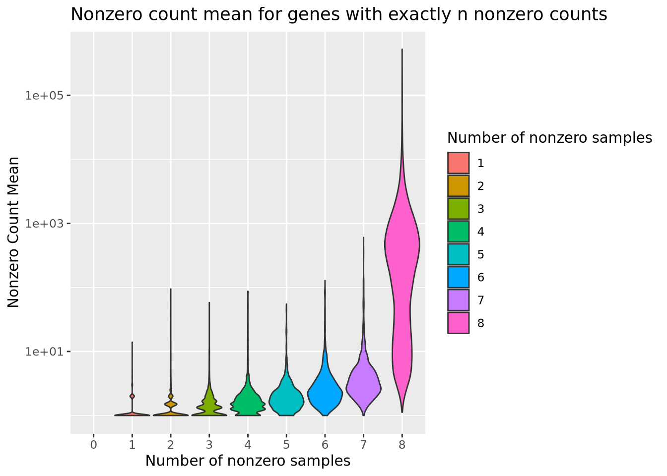
From this plot, we see that the mean count for genes with even a single sample with a zero is substantially lower than most genes without any zeros. We might therefore decide to filter out genes that have any zeros, with the rationale that most genes of appreciable abundance would still be included. However, there are some genes with a high average count for samples that are not zero that would be eliminated if we chose to use only genes expressed in all 8 samples. Again, there is no clear choice of filtering threshold, and a subjective decision is necessary.
One important property of RNASeq expression data is that genes with higher mean count also have higher variance. This mean-variance dependence means these count data are heteroskedastic, a term used to describe data that has inconstant variance across different values. We can visualize this dependence by calculating the mean and variance for each of our normalized count genes and plotting them against each other:
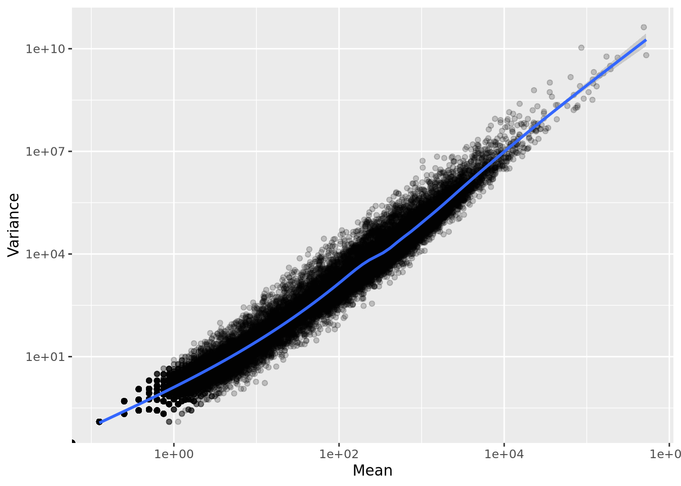
Unlike in microarray data, where probesets can be filtered based on variance, using low variance as a filter for count data would result in filtering out genes with low mean, which would lead to undesirable bias toward highly expressed genes.
Depending on the experiment, it may be meaningful if a gene is detected at all in any of the samples. In these cases, genes with only 1 read in a single sample might be kept, even though these genes would not result in confident statistical inference if subjected to differential expression. The scientific question asked by the experiment is an important consideration when deciding thresholds.
When the goal of the RNASeq experiment is differential expression analysis, a good rule of thumb when choosing a filtering threshold is to choose genes that have sufficiently many non-zero counts such that the statistical method has enough variance to perform reliable inference. For example, a reasonable filtering threshold might be to include genes that have non-zero counts in at least 50% of the samples. This threshold depends only upon the number of samples being considered. In an experimental design with two or more sample groups, a reasonable strategy might be to require at least 50% of samples within at least one group or within all groups to be included. Taking the experimental design into account when filtering can ensure the most interesting genes, e.g. those expressed only in one condition, are captured.
Regardless of the filtering strategy used, there is no biological meaning to any filtering threshold. The number of reads detected for each gene is dependent primarily upon the library size, where larger libraries are more likely to sample lowly abundant genes. Therefore, we cannot filter genes with the intent of “removing lowly expressed genes”; instead we can only filter out genes that are below the detection threshold afforded by the library size of the dataset.
8.7.8 Count Distributions
The range of gene expression in a cell varies by orders of magnitude. The following histogram plots the distribution of read count values for one of the adult samples:
dplyr::select(filtered_counts, Ad_1) %>%
  mutate(`log10(counts+1)`=log10(Ad_1+1)) %>%
  ggplot(aes(x=`log10(counts+1)`)) +
  geom_histogram(bins=50) +
  labs(title='log10(counts) distribution for Adult mouse')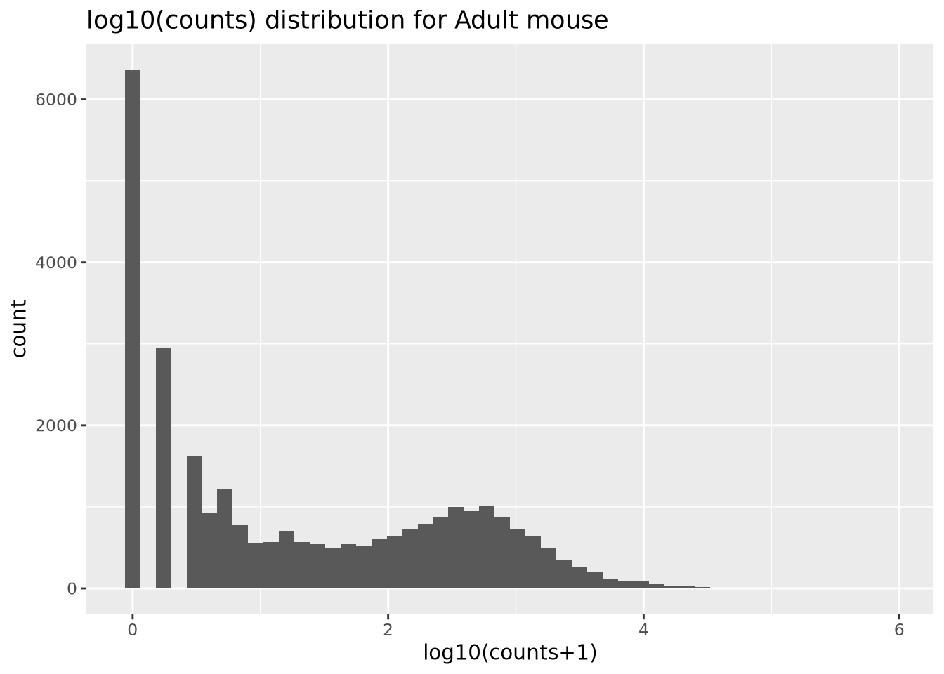
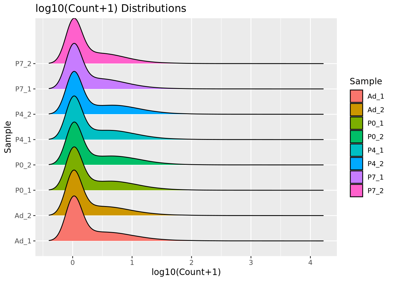
We add 1 count, called a pseudocount, to avoid taking the log of zero, therefore all the genes at \(x=0\) are genes that have no reads. From the plot, the largest count is nearly \(10^6\) while the smallest is 1, spanning nearly six orders of magnitude. There are relatively few of these highly abundant genes, however, and most genes are betwen the range of 100-10,000 reads. We see that this distribution is similar for all the samples, when displayed as a ridgeline plot:
library(ggridges)

pivot_longer(filtered_counts,-c(gene),names_to="Sample",values_to="Count") %>%
  mutate(`log10(Count+1)`=log10(Count+1)) %>%
  ggplot(aes(y=Sample,x=`log10(Count+1)`,fill=Sample)) +
  geom_density_ridges(bandwidth=0.132) +
  labs(title="log10(Count+1) Distributions")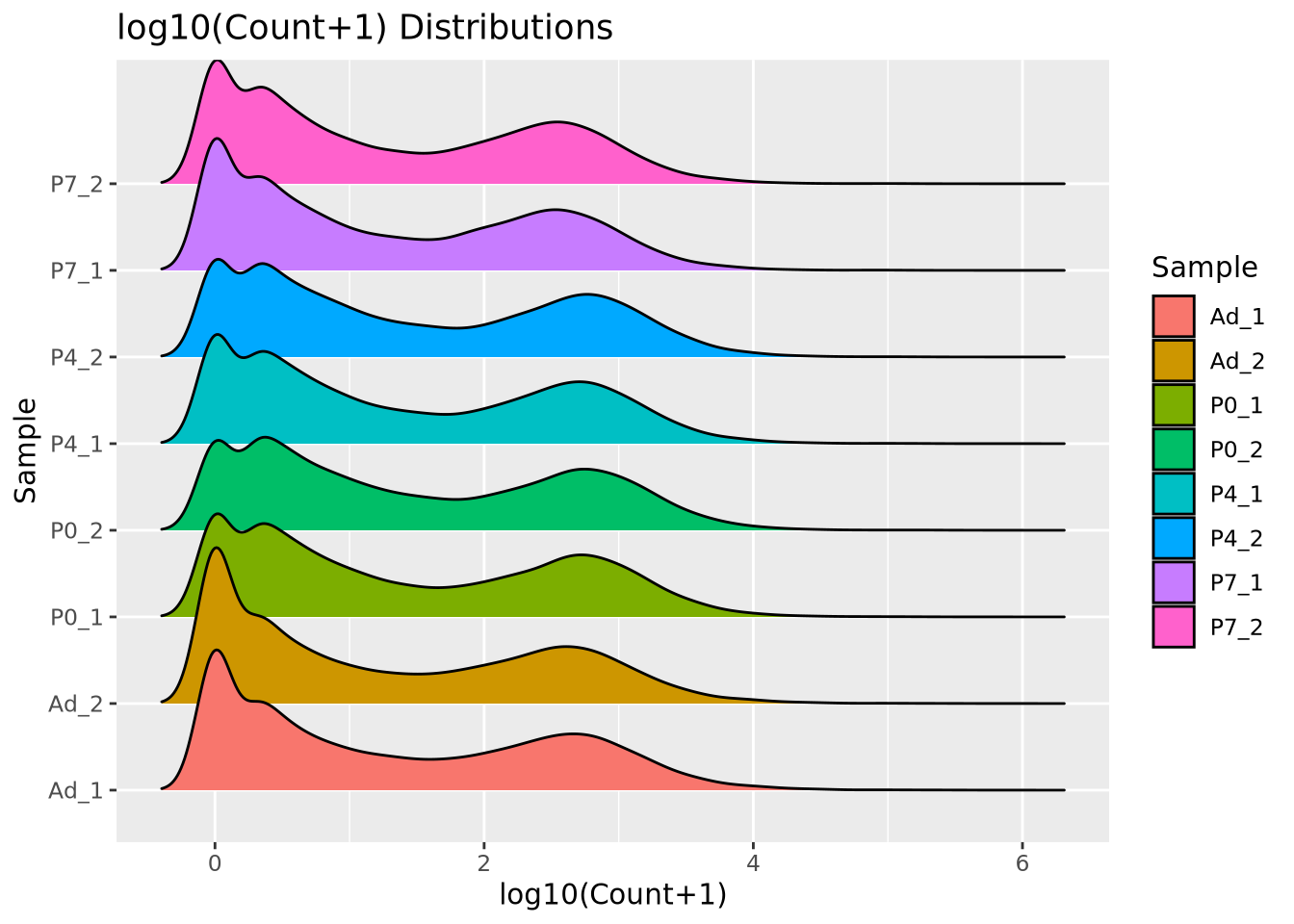
The general shape of the distributions is similar, with a large mode of counts at zero, representing genes that had zero counts in that sample, and a wider mode between 100 and 10,000 where most consistently expressed genes fall. However, we note that the peak count of these larger modes vary and also recall that though the difference appears small, the log scale of the x axis means the differences in counts may be substantial. We will discuss the implications of this in the next section.
8.7.8.1 Count Normalization
The number of reads generated for each sample in an RNASeq dataset varies from sample to sample due to randomness in the biochemical process that generates the data. The relationship between the number of reads that maps to any given gene and the relative abundance of the molecule in the sample is dependent upon the library size of each sample. The direct number of counts, or the raw counts, is therefore not directly comparable between samples. A simple example should suffice to make this clear:
Imagine two RNASeq datasets generated from the same RNA sample. One of the samples was sequenced to 1000 reads, and the other to 2000 reads. Now imagine that one gene makes up half of the RNA in the original sample. In the sample with 1000 reads, we find this gene has 500 reads. In the sample with 2000 reads, the gene has 1000 of those reads. In both cases the fraction of reads that map to the gene is 0.5, but the absolute number of reads differs greatly. This is why the raw counts for a gene are not directly comparable between samples with different numbers of reads. Since in general every sample will have a unique number of reads, these raw counts will never be directly comparable. The way we mitigate this problem is with a statistical procedure called count normalization.
Count normalization is the process by which the number of raw counts in each sample is scaled by a factor to make multiple samples comparable. Many strategies have been proposed to do this, but the simplest is a family of methods that divide by some factor of the library size. A common method in this family is to compute counts per million reads or CPM normalization, which scales each gene count by the number of millions of reads in the library:
\[ cpm_{s,i} = \frac{c_{s,i}}{l_s} * 10^6 \]
Here, \(c_{s,i}\) is the raw count of gene \(i\) in sample \(s\), and \(l_s\) is the number of reads in the dataset for sample \(s\). If each sample is scaled by their own library size, then in principle the proportion of read counts assigned to each gene out of all reads for that sample will be comparable across samples. When we have no additional knowledge of the distribution of genes in our system, library size normalization methods are the most general and make the fewest assumptions. Below is a ridgeline plot of the counts distribution after CPM normalization:
The distributions look quite different after CPM normalization, but the modes now look more consistent than with raw counts.
One drawback of library size normalization is it is sensitive to extreme values; individual genes with many more reads in one sample than in other samples. These outliers can lead to pathological effects when comparing gene count values across samples. However, if we are measuring gene expression in a single biological system like mouse or human, as is often the case, other methods have been developed to better use our understanding of the gene expression distribution to perform more robust and biologically meaningful normalization. A more robust approach is possible when we make the reasonable assumption that, for any set of biological conditions in an experiment, most genes are not differentially expressed. This is the assumption made by the DESeq2 normalization method.
The DESeq2 normalization method is a statistical procedure that uses the median geometric mean computed across all samples to determine the scale factor for each sample. The procedure is somewhat complicated and we encourage the reader to examine it in detail in the DESeq2 publication (Love, Huber, and Anders 2014). The method has proven to be consistent and reliable compared with other strategies (Dillies et al. 2013) and is the default normalization for the populare DESeq2 differential expression method, which will be described in a later section. The DESeq2 normalization method may be implemented using the DESeq2 Bioconductor package:
library(DESeq2)
# DESeq2 requires a counts matrix, column data (sample information), and a formula
# the counts matrix *must be raw counts*
count_mat <- as.matrix(filtered_counts[-1])

row.names(count_mat) <- filtered_counts$gene

dds <- DESeqDataSetFromMatrix(
  countData=count_mat,
  colData=tibble(sample_name=colnames(filtered_counts[-1])),
  design=~1 # no formula is needed for normalization, ~1 produces a trivial design matrix
)

# compute normalization factors
dds <- estimateSizeFactors(dds)

# extract the normalized counts
deseq_norm_counts <- as_tibble(counts(dds,normalized=TRUE)) %>%
  mutate(gene=filtered_counts$gene) %>%
  relocate(gene)
Using the DESeq2 package, we first construct a DESeq object using the raw counts
matrix, a sample information tibble with only a sample name column, and a
trivial design formula, which will be explained in more depth in the
DESeq2/edgeR section. The estimateSizeFactors() function performs the
normalization routine on the counts, and the counts(dds,normalized=TRUE) call
extracts the normalized counts matrix. When plotted as a ridgeline plot as
before, we see that the gene expression distribution modes are better behaved
compared to raw counts, and the shape of the distribution is preserved unlike
with CPM normalized counts:
pivot_longer(deseq_norm_counts,-c(gene),names_to="Sample",values_to="Count") %>%
  mutate(`log10(Count+1)`=log10(Count+1)) %>%
  ggplot(aes(y=Sample,x=`log10(Count+1)`,fill=Sample)) +
  geom_density_ridges(bandwidth=0.132) +
  labs(title="log10(Count+1) Distributions")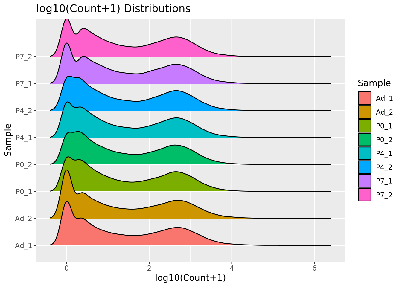
The DESeq2 normalization procedure has two important considerations to keep in mind:
- The procedure borrows information across all samples. The geometric mean of counts across all samples is computed as part of the normalization procedure. This means that the size factors computed depend on the samples in the dataset. The normalized counts for one sample will likely change if it is normalized with a different set of samples.
- The procedure does not use genes with any zero counts. The geometric mean calculation across all samples means that any sample with a zero count results in the entire geometric mean being zero. For this reason only genes with nonzero counts in every sample are used to calculate the normalization factors. If one of the samples has a large number of zeros, for example due to a small library size, this could dramatically influence the normalization factors for the entire experiment.
The CPM normalization procedure does not borrow information across all samples, and therefore is not subject to these considerations.
These are only two of many possible normalization methods, DESeq2 being the most popular at the time of writing. For a detailed explanation of many normalization methods, see (Dillies et al. 2013).
8.7.8.2 Count Transformation
As mentioned in the Count Data section, one way to deal with the non-normality
of count data is to perform a data transformation that makes the counts data
follow a normal distribution. Transformation to normality allows common and
powerful statistical methods like linear regression to be used. The most basic
count transformation is to take the logarithm of the counts. However, this can
be problematic for genes with low counts, causing the values to spread further
apart than genes with high counts, increasing the likelihood of false positive
results. To address this issue, the DESeq2 package provides the rlog()
function that performs a regularized logarithmic transformation that adjusts the
log transform based on the mean count of each gene.
The rlog transformation also has the desirable effect of making the count data homoskedastic, meaning the variance of a gene is not dependent on the mean. Some statistical methods assume that a dataset has this property. The relationship of mean count vs variance will be discussed in more detail in the next section.
We can clearlysee the effect of rlog on the counts distribution by plotting the rlog’ed counts using a ridgeline plot as before:
# the dds is the DESeq2 object from earlier
rld <- rlog(dds)

# extract rlog values as a tibble
rlog_counts <- as_tibble(assay(rld))
rlog_counts$gene <- filtered_counts$gene
pivot_longer(rlog_counts,-c(gene),names_to="Sample",values_to="rlog count") %>%
  ggplot(aes(y=Sample,x=`rlog count`,fill=Sample)) +
  geom_density_ridges(bandwidth=0.132) +
  labs(title="rlog Distributions")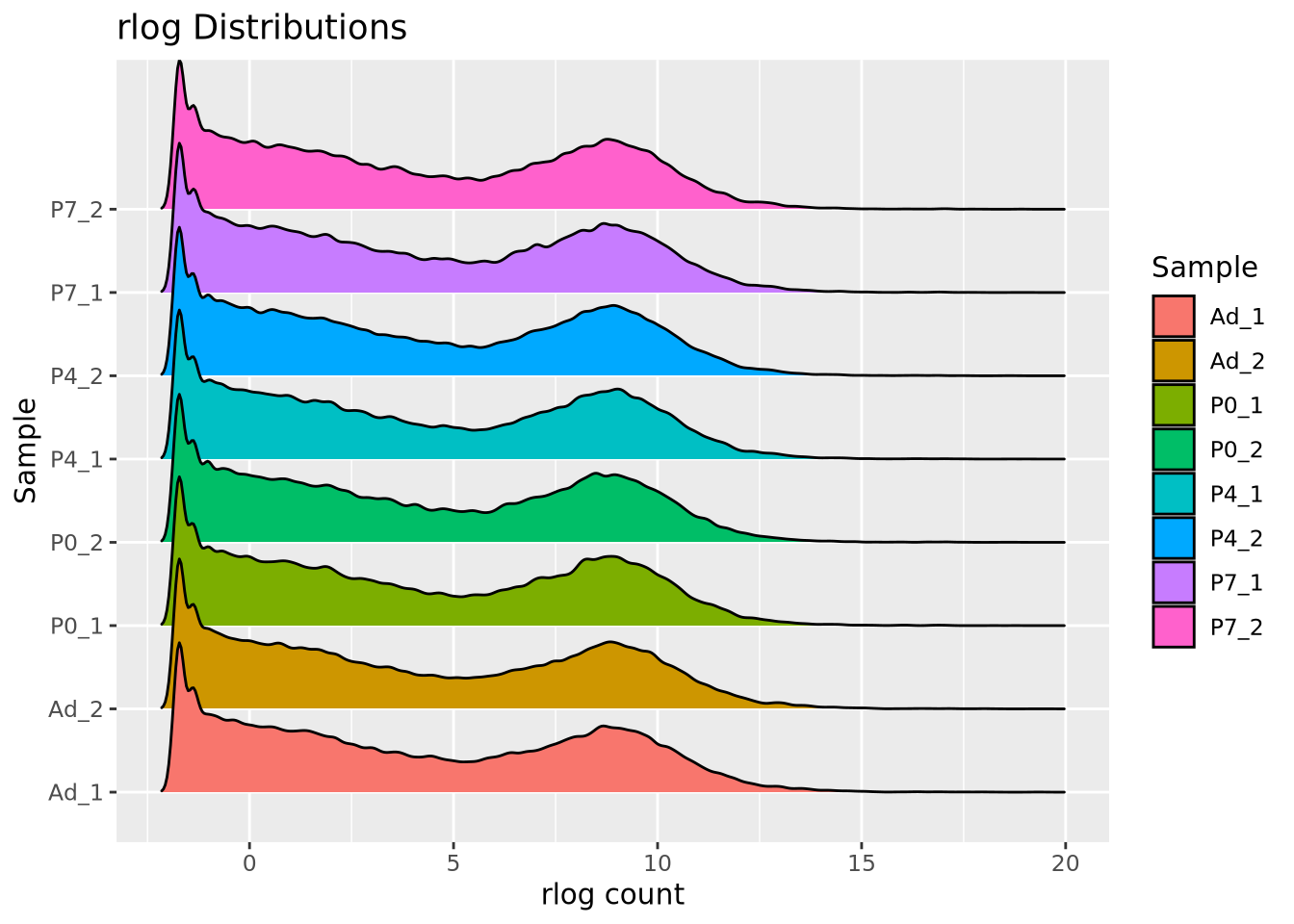
It is generally accepted that count transformations have significant drawbacks compared with statistical methods that model counts and errors explicitly, like generalized linear models (GLM) such as Poisson and Negative Binomial regressions (St-Pierre, Shikon, and Schneider 2018). Whenever possible, these GLM based methods should be used instead of transformations. However, the transformations may sometimes be necessary depending on the required analysis, so the rlog function in DESeq2 may be useful for these cases.
8.7.9 Differential Expression: RNASeq
The read counts for each gene or transcript form the primary data used to identify genes whose expression correlates with some condition of interest. The counts matrix created by concatenating read counts for all genes across a set of samples where rows are genes or transcripts and columns are samples is the most common form of expression data used for this purpose. As mentioned in the Count Data section, these counts are not normally distributed and therefore require a statistical approach that can accommodate the counts distribution.
The strong relationship between the mean and variance is characteristic of RNASeq expression data, and motivates the use of a generalized linear model called negative binomial regression. Negative binomial regression models count data using the negative binomial distribution, which allows the relationship of mean and variance of a counts distribution to vary. The statistical details of the negative binomial distribution and negative binomial regression are beyond the scope of this book, but below we will discuss the aspects necessary to implement differential expression analysis.
8.7.9.1 DESeq2/EdgeR
DESeq2 and edgeR are bioconductor packages that both implement negative binomial regression to perform differential expression on RNASeq data. Both perform raw counts normalization as part of their function, though they differ in the normalization method (DESeq2 method is described above, while edgeR uses trimmed mean of M-values (TMM), see (Robinson and Oshlack 2010)). The interface for using both packages is also similar, so we will focus on DESeq2 in this section.
As mentioned briefly above, DESeq2 requires three pieces of information to perform differential expression:
- A raw counts matrix with genes as rows and samples as columns
- A data frame with metadata associated with the columns
- A design formula for the differential expression model
DESeq2 requires raw counts due to its normalization procedure, which borrows information across samples when computing size factors, as described above in the Count Normalization section.
With these three pieces of information, we construct a DESeq object:
library(DESeq2)

# filter counts to retain genes with at least 6 out of 8 samples with nonzero counts
filtered_counts <- counts[rowSums(counts[-1]!=0)>=6,]

# DESeq2 requires a counts matrix, column data (sample information), and a formula
# the counts matrix *must be raw counts*
count_mat <- as.matrix(filtered_counts[-1])
row.names(count_mat) <- filtered_counts$gene

# create a sample matrix from sample names
sample_info <- tibble(
  sample_name=colnames(filtered_counts[-1])
) %>%
  separate(sample_name,c("timepoint","replicate"),sep="_",remove=FALSE) %>%
  mutate(
    timepoint=factor(timepoint,levels=c("Ad","P0","P4","P7"))
  )

design <- formula(~ timepoint)

sample_info
## # A tibble: 8 x 3
## sample_name timepoint replicate
## <chr> <fct> <chr>
## 1 P0_1 P0 1
## 2 P0_2 P0 2
## 3 P4_1 P4 1
## 4 P4_2 P4 2
## 5 P7_1 P7 1
## 6 P7_2 P7 2
## 7 Ad_1 Ad 1
## 8 Ad_2 Ad 2The design formula ~ timepoint is similar to that supplied to the
model.matrix() function as described in the Differential Expression Analysis
section, where DESeq2 implicitly creates the model matrix by combining the
column data with the formula. In this differential expression analysis, we wish
to identify genes that are different between the timepoints P0, P4, P7,
and Ad. With these three pieces of information prepared, we can create a DESeq
object and perform differential expression analysis:
dds <- DESeqDataSetFromMatrix(
  countData=count_mat,
  colData=sample_info,
  design=design
)
dds <- DESeq(dds)
resultsNames(dds)
## [1] "Intercept" "timepoint_P0_vs_Ad" "timepoint_P4_vs_Ad"
## [4] "timepoint_P7_vs_Ad"DESeq2 performed differential expression on each gene and estimated parameters
for three different comparisons - P0 vs Ad, P4 vs Ad, and P7 vs Ad. Here, Ad is
the reference group so that we may interpret the statistics as relative to the
adult animals. The choice of reference group does not change the magnitude of
the results, but may change the sign of the estimated coefficients, which are
log2 fold changes. To extract out the differential expression statistics for the
P0 vs Ad comparison, we can use the results() function:
res <- results(dds, name="timepoint_P0_vs_Ad")
p0_vs_Ad_de <- as_tibble(res) %>%
  mutate(gene=rownames(res)) %>%
  relocate(gene) %>%
  arrange(pvalue)
p0_vs_Ad_de
## # A tibble: 21,213 x 7
## gene baseMean log2FoldChange lfcSE stat pvalue padj
## <chr> <dbl> <dbl> <dbl> <dbl> <dbl> <dbl>
## 1 ENSMUSG00000000031.17 19624. 6.75 0.190 35.6 5.70e-278 1.07e-273
## 2 ENSMUSG00000026418.17 9671. 9.84 0.285 34.5 2.29e-261 2.15e-257
## 3 ENSMUSG00000051855.16 3462. 5.35 0.157 34.1 2.84e-255 1.77e-251
## 4 ENSMUSG00000027750.17 9482. 4.05 0.125 32.4 2.26e-230 1.06e-226
## 5 ENSMUSG00000042828.13 3906. -5.32 0.167 -31.8 1.67e-221 6.25e-218
## 6 ENSMUSG00000046598.16 1154. -6.08 0.197 -30.8 4.77e-208 1.49e-204
## 7 ENSMUSG00000019817.19 1952. 5.15 0.171 30.1 1.43e-198 3.83e-195
## 8 ENSMUSG00000021622.4 17146. -4.57 0.157 -29.0 4.41e-185 1.03e-181
## 9 ENSMUSG00000002500.16 2121. -6.20 0.217 -28.5 6.69e-179 1.39e-175
## 10 ENSMUSG00000024598.10 1885. 5.90 0.209 28.2 5.56e-175 1.04e-171
## # ... with 21,203 more rowsThese are the results of the differential expression comparing P0 with Ad; the
other contrasts (P4 vs Ad and P7 vs Ad) may be extracted by specifying the
appropriate result names to the name argument to the results() function. The columns in the DESeq2 results are defined as follows:
- baseMean - the mean normalized count of all samples for the gene
- log2FoldChange - the estimated coefficient (i.e. log2FoldChange) for the comparison of interest
- lfcSE - the standard error for the log2FoldChange estimate
- stat - the Wald statistic associated with the log2FoldChange estimate
- pvalue - the nominal p-value of the Wald test (i.e. the signifiance of the association)
- padj - the multiple testing adjusted p-value (i.e. false discovery rate)
In the P0 vs Ad comparison, we can check the number of significant results easily:
# number of genes significant at FDR < 0.05
filter(p0_vs_Ad_de,padj<0.05)
## # A tibble: 7,557 x 7
## gene baseMean log2FoldChange lfcSE stat pvalue padj
## <chr> <dbl> <dbl> <dbl> <dbl> <dbl> <dbl>
## 1 ENSMUSG00000000031.17 19624. 6.75 0.190 35.6 5.70e-278 1.07e-273
## 2 ENSMUSG00000026418.17 9671. 9.84 0.285 34.5 2.29e-261 2.15e-257
## 3 ENSMUSG00000051855.16 3462. 5.35 0.157 34.1 2.84e-255 1.77e-251
## 4 ENSMUSG00000027750.17 9482. 4.05 0.125 32.4 2.26e-230 1.06e-226
## 5 ENSMUSG00000042828.13 3906. -5.32 0.167 -31.8 1.67e-221 6.25e-218
## 6 ENSMUSG00000046598.16 1154. -6.08 0.197 -30.8 4.77e-208 1.49e-204
## 7 ENSMUSG00000019817.19 1952. 5.15 0.171 30.1 1.43e-198 3.83e-195
## 8 ENSMUSG00000021622.4 17146. -4.57 0.157 -29.0 4.41e-185 1.03e-181
## 9 ENSMUSG00000002500.16 2121. -6.20 0.217 -28.5 6.69e-179 1.39e-175
## 10 ENSMUSG00000024598.10 1885. 5.90 0.209 28.2 5.56e-175 1.04e-171
## # ... with 7,547 more rowsThere were 7,557 significantly differentially expressed genes associated with this comparison, which includes both up- and down-regulated genes (examine the signs of the log2FoldChange column). A common diagnostic plot of differenial expression results is the so-called volcano plot which plots the log2FoldChange on the x-axis against -log10 adjusted p-value on the y-axis:
mutate(
  p0_vs_Ad_de,
  `-log10(adjusted p)`=-log10(padj),
  `FDR<0.05`=padj<0.05
  ) %>%
  ggplot(aes(x=log2FoldChange,y=`-log10(adjusted p)`,color=`FDR<0.05`)) +
  geom_point()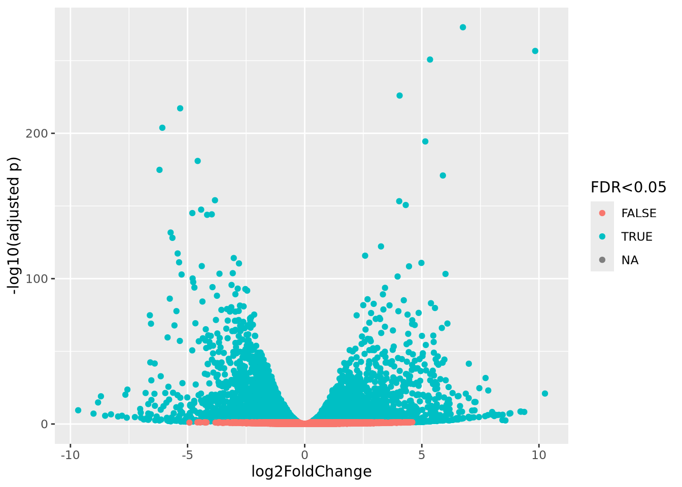
The plot shows that there are significant genes at FDR < 0.05 that are increased and decreased in the comparison.
DESeq2 has many capabilities beyond this basic differential expression functionality as described in its comprehensive documentation in its vignette.
As mentioned, edgeR implements a very similar model to DESeq2 and also has excellent documentation.
8.7.9.2 limma/voom
While the limma package was initially developed for microarray analysis, the authors added support for RNASeq soon after the HTS technique became available. limma accommodates count data by first performing a Count Transformation using its own voom transformation procedure. voom transforms counts by first performing a counts per million normalization, taking the logarithm of the CPM values, and finally estimates the mean-variance relationship across genes for use in its empirical Bayes statistical framework. The counts data being thus transformed, limma performs statistical inference using its usual linear model framework to produce differential expression results with arbitrarily complex statistical models.
This brief example is from the limma User Guide chapter 15, and covers loading and processing data from an RNA-seq experiment. We go into more depth while working with limma in assignment 6.
Without going into too much detail, the design variable is how we inform limma
of our experimental conditions, and where limma draws from to construct its
linear models correctly. This design is relatively simple, just four samples
belonging to two different conditions (the swirls here refer to the swirl of
zebra fish, you can just see them as a phenotypic difference)
design <- data.frame(swirl = c("swirl.1", "swirl.2", "swirl.3", "swirl.4"),
                     condition = c(1, -1, 1, -1))
dge <- DGEList(counts=counts)
keep <- filterByExpr(dge, design)
dge <- dge[keep,,keep.lib.sizes=FALSE]
DGEList() is a function from edgeR, of which limma borrows some loading and
filtering functions. This experiment filters by expression level, and uses
square bracket notation ([]) to reduce the number of rows.
Finally, the expression data is transformed into CPM, counts per million, and
a linear model is applied to the data with lmFit(). topTable() is used to view the most
differentially expressed data.
# limma trend
logCPM <- cpm(dge, log=TRUE, prior.count=3)
fit <- lmFit(logCPM, design)
fit <- eBayes(fit, trend=TRUE)
topTable(fit, coef=ncol(design))