- Syllabus
- 1 Introduction
- 2 Data in Biology
- 3 Preliminaries
- 4 R Programming
- 4.1 Before you begin
- 4.2 Introduction
- 4.3 R Syntax Basics
- 4.4 Basic Types of Values
- 4.5 Data Structures
- 4.6 Logical Tests and Comparators
- 4.7 Functions
- 4.8 Iteration
- 4.9 Installing Packages
- 4.10 Saving and Loading R Data
- 4.11 Troubleshooting and Debugging
- 4.12 Coding Style and Conventions
- 4.12.1 Is my code correct?
- 4.12.2 Does my code follow the DRY principle?
- 4.12.3 Did I choose concise but descriptive variable and function names?
- 4.12.4 Did I use indentation and naming conventions consistently throughout my code?
- 4.12.5 Did I write comments, especially when what the code does is not obvious?
- 4.12.6 How easy would it be for someone else to understand my code?
- 4.12.7 Is my code easy to maintain/change?
- 4.12.8 The
stylerpackage
- 5 Data Wrangling
- 6 Data Science
- 7 Data Visualization
- 8 Biology & Bioinformatics
- 8.1 R in Biology
- 8.2 Biological Data Overview
- 8.3 Bioconductor
- 8.4 Microarrays
- 8.5 High Throughput Sequencing
- 8.6 Gene Identifiers
- 8.7 Gene Expression
- 8.7.1 Gene Expression Data in Bioconductor
- 8.7.2 Differential Expression Analysis
- 8.7.3 Microarray Gene Expression Data
- 8.7.4 Differential Expression: Microarrays (limma)
- 8.7.5 RNASeq
- 8.7.6 RNASeq Gene Expression Data
- 8.7.7 Filtering Counts
- 8.7.8 Count Distributions
- 8.7.9 Differential Expression: RNASeq
- 8.8 Gene Set Enrichment Analysis
- 8.9 Biological Networks .
- 9 EngineeRing
- 10 RShiny
- 11 Communicating with R
- 12 Contribution Guide
- Assignments
- Assignment Format
- Starting an Assignment
- Assignment 1
- Assignment 2
- Assignment 3
- Problem Statement
- Learning Objectives
- Skill List
- Background on Microarrays
- Background on Principal Component Analysis
- Marisa et al. Gene Expression Classification of Colon Cancer into Molecular Subtypes: Characterization, Validation, and Prognostic Value. PLoS Medicine, May 2013. PMID: 23700391
- Scaling data using R
scale() - Proportion of variance explained
- Plotting and visualization of PCA
- Hierarchical Clustering and Heatmaps
- References
- Assignment 4
- Assignment 5
- Problem Statement
- Learning Objectives
- Skill List
- DESeq2 Background
- Generating a counts matrix
- Prefiltering Counts matrix
- Median-of-ratios normalization
- DESeq2 preparation
- O’Meara et al. Transcriptional Reversion of Cardiac Myocyte Fate During Mammalian Cardiac Regeneration. Circ Res. Feb 2015. PMID: 25477501l
- 1. Reading and subsetting the data from verse_counts.tsv and sample_metadata.csv
- 2. Running DESeq2
- 3. Annotating results to construct a labeled volcano plot
- 4. Diagnostic plot of the raw p-values for all genes
- 5. Plotting the LogFoldChanges for differentially expressed genes
- The choice of FDR cutoff depends on cost
- 6. Plotting the normalized counts of differentially expressed genes
- 7. Volcano Plot to visualize differential expression results
- 8. Running fgsea vignette
- 9. Plotting the top ten positive NES and top ten negative NES pathways
- References
- Assignment 6
- Assignment 7
- Appendix
- A Class Outlines
6.5 Network Analysis .
What is a network? What is network analysis? What are some example network analysis applications in biology and bioinformatics (there is a full ksection on [Biological Networks] in the bio chapter, these are just illustrative examples)? How do we represent networks in R, and how do we analyze them? (Network visualization is covered in the data viz chapter, might be helpful to write these two sections together)
library(igraph)The basic components of a network are vertex (or node), which is the features or subjects we are interested in. The edges are connections between the vertices. In a general context, one example is the relationship network. The vertices are people. If two people are friends, we draw an edge to connect them. In a biology context, the vertices may be genes, and edges represent whether there are any correlations between two genes.
Vertices and edges can have attributes. For example, in a social interaction network, we may assign different colors to the vertices according to a student’s major. When connect two students when they know each other, we can also assign weights to the edges to represent how often they interact with each other.
A cyclic network has at least one directed path that starts and ends in the same node.
set.seed(2)
samp_g <- sample_gnm(n = 4, m = 4)
vertex_attr(samp_g) <- list(color = rep("slategray1", gorder(samp_g)))
plot(samp_g)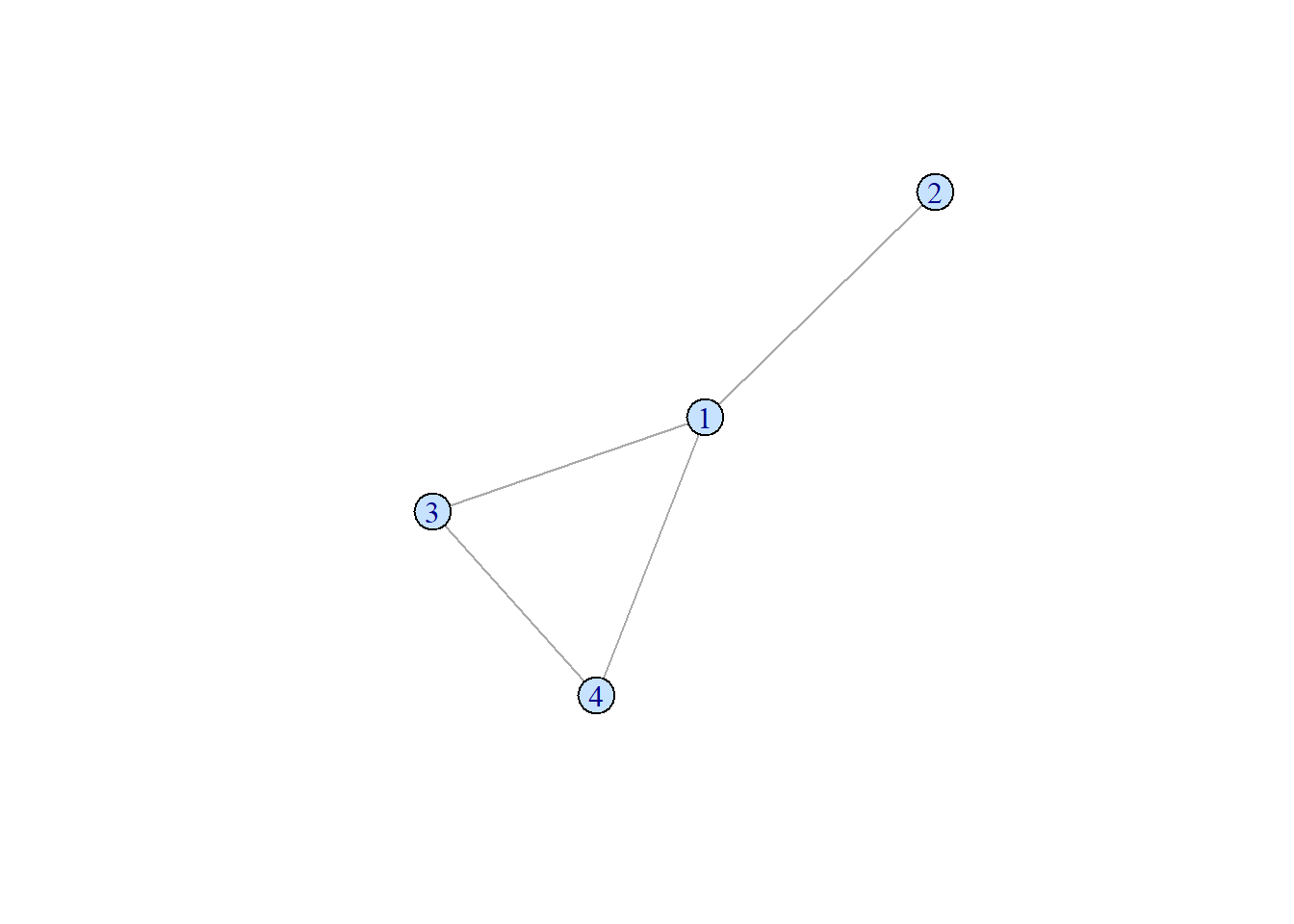
An acyclic network , on the other hand, does not have any cycle path.
set.seed(1)
samp_g <- sample_gnm(n = 5, m = 4)
vertex_attr(samp_g) <- list(color = rep("slategray1", gorder(samp_g)))
plot(samp_g)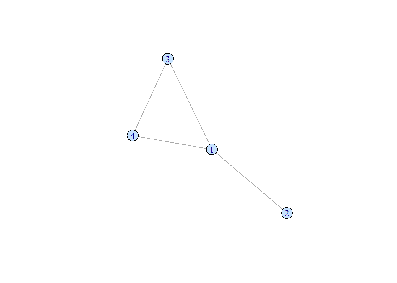
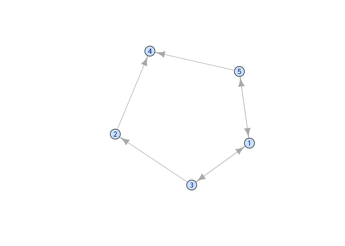
The edges in a directed network point to one specific direction. (But, there can be double-headed arrows!) One common example is a network representing cell metabolic process.
set.seed(2)
samp_g <- sample_gnm(n = 5, m = 7, directed = TRUE)
vertex_attr(samp_g) <- list(color = rep("slategray1", gorder(samp_g)))
plot(samp_g)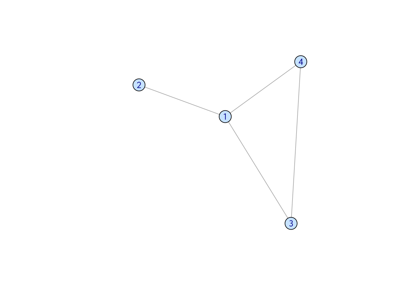
The edges in a indirect network do not have direction. Common examples include social interaction network and gene correlation network.
set.seed(3)
samp_g <- sample_gnm(n = 5, m = 7, directed = FALSE)
vertex_attr(samp_g) <- list(color = rep("slategray1", gorder(samp_g)))
plot(samp_g)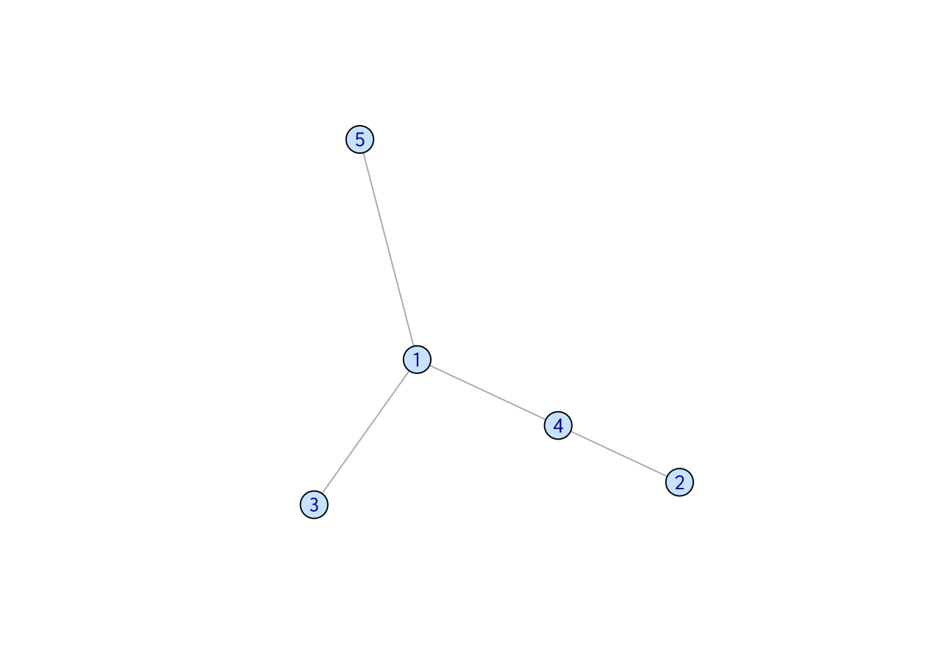
6.5.1 Basic network analysis
6.5.1.1 Shortest path
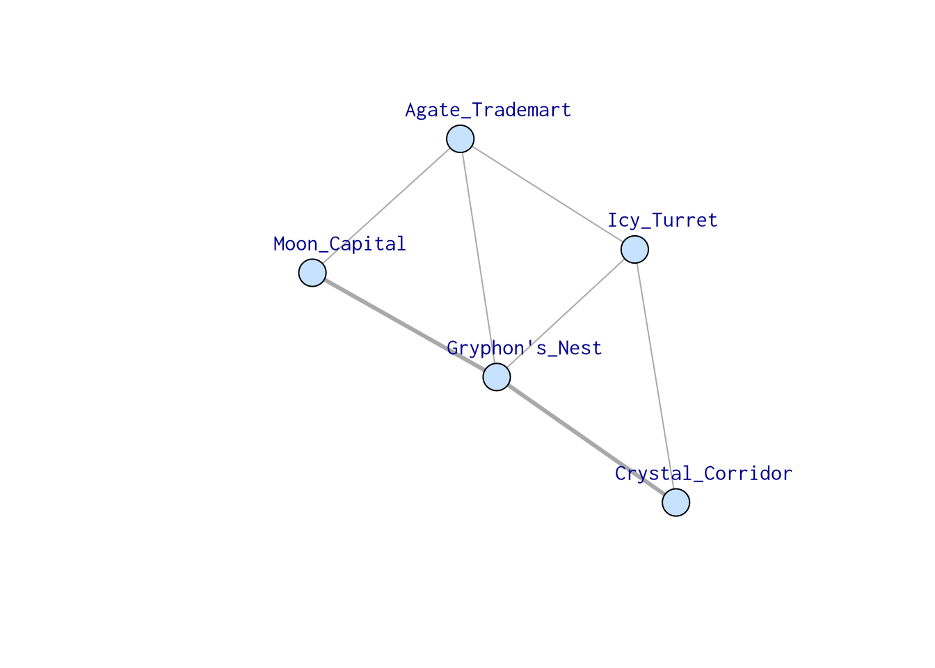
The shortest path between two vertices is… yes, the shortest path you can go from one vertex to the other. There may be more than one shortest paths between two vertices.
In the following network, there are many ways to go from “Moon_Capital” to “Crystal_Corridor,” but there’s only one shortest path, which is “Moon_Capital” -> “Gryphon’s_Nest” -> “Crystal_Corridor.” On the other hand, when you want to go from “Moon_Capital” to “Icy_Turret,” there are two possible ways: one through “Gryphon’s_Nest,” one through “Agate_Trademart.”
In igraph, this can be calculated using shortest_paths().
shortest_paths(samp_g, from = "Moon_Capital", to = "Crystal_Corridor")$vpath## [[1]]
## + 3/5 vertices, named, from 6b2bdd0:
## [1] Moon_Capital Gryphon's_Nest Crystal_CorridorOne thing to keep in mind is, when weights are assigned to edges and being considered, the shortest path may not be the path that goes through the least number of vertices. In this example, consider the weight assigned to the edge connecting “Moon_Capital” and “Gryphon’s_Nest” is substantially large. The Royal Priest warned you that Gryphons live at the top of the hill, and it’s too hard to climb.
Let’s color the edges according to their weights. Green means 1, blue means 2 while red means 3. Now, the shortest path from “Moon_Capital” to “Crystal_Corridor” becomes “Moon_Capital” -> “Agate_Trademart” -> “Icy_Turret” -> “Crystal_Corridor.”
set.seed(4)
names <- c("Moon_Capital", "Icy_Turret", "Crystal_Corridor", "Gryphon's_Nest", "Agate_Trademart")
samp_g <- sample_gnm(n = 5, m = 7)
vertex_attr(samp_g) <- list(name = names, color = rep("slategray1", gorder(samp_g)))
edge_attr(samp_g) <- list(
  color = c("deepskyblue", "salmon", "deepskyblue", "deepskyblue", "palegreen3", "palegreen3", "salmon"),
  weights = c(2, 3, 2, 2, 1, 1, 3)
)
plot(samp_g,
  vertex.label.cex = 1,
  vertex.label.dist = 3, edge.width = c(3, 1, 1, 1, 3, 3, 1)
)
We can conveniently find the shortest path with weights assigned!
shortest_paths(samp_g,
  from = "Moon_Capital", to = "Crystal_Corridor",
  weights = edge_attr(samp_g, "weights")
)$vpath
## [[1]]
## + 4/5 vertices, named, from 6b4e4d4:
## [1] Moon_Capital Agate_Trademart Icy_Turret Crystal_Corridor6.5.1.2 Vertex centrality
The degree of a vertex is the number of edges connected to it. In igraph, this can be calculated using degree().
g <- graph_from_data_frame(data.frame(
  "from" = c("A", "A", "A", "A", "A", "B", "C", "A", "G", "H", "H", "H", "H", "H", "M", "I", "G", "N", "N"),
  "to" = c("B", "C", "D", "E", "F", "D", "E", "G", "H", "I", "J", "K", "L", "M", "K", "J", "N", "O", "P")
), directed = F)
vertex_attr(g) <- list(name = vertex_attr(g, "name"), color = rep("slategray1", gorder(g)))
plot(g)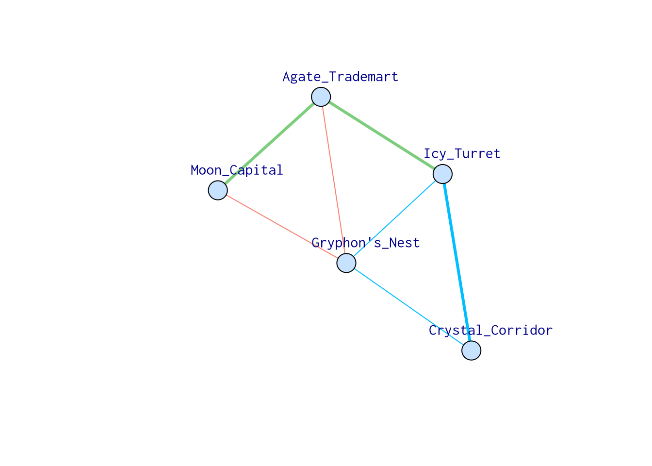
degree(g)## A B C G H M I N D E F J K L O P
## 6 2 2 3 6 2 2 3 2 2 1 2 2 1 1 1The centrality of a vertex indicates how important it is in a network. For instance, after seeing a social interaction network, one question we can ask is “which person has the most influential power in this community?” There are many different types of centrality, here we will only go through the basics.
To some extent, the degree can be used to evaluate the importance of a vertex. When a vertex is connected to a lot of other vertices, it naturally appears to be more important and has more ability to pass down information to other vertices. Assume you just opened a new on-line shop and you want to attract new customers as many as possible, you start by reaching out to the person you know has the largest number of friends.
But, sometimes, people with the largest number of friends may not necessarily be the one who can “spread the word” to the whole community the most efficiently. In the example above, although A and H have a lot of connections, in fact, it seems like if we pass an information to G, the whole community will be influenced the most quickly.
This leads us to closeness centrality, which is the sum of the length of the shortest paths between a node and all the other nodes in the graph. Although A and H have a lot of friends, it takes too long to reach the other side of the graph. When we calculating the closeness centrality using closeness() function to calculate closeness centrality.
closeness(g)## A B C G H M I
## 0.03225806 0.02272727 0.02272727 0.03703704 0.03225806 0.02272727 0.02272727
## N D E F J K L
## 0.02702703 0.02272727 0.02272727 0.02222222 0.02272727 0.02272727 0.02222222
## O P
## 0.01960784 0.01960784Betweenness centrality is the number of shortest paths that pass through the vertex. In this example, G is the also the one with the highest betweenness centrality.
betweenness(g)## A B C G H M I N D E F J K L O P
## 58 0 0 72 58 0 0 27 0 0 0 0 0 0 0 06.5.2 Create your own
Check the network visualization section to see a more detailed illustration about how to create your own network from scratch, and how to customize it!