8.5 High Throughput Sequencing

High throughput sequencing (HTS) technologies measure and digitize the nucleotide sequences of thousands to billions of DNA molecules simultaneously. In contrast to microarrays, which cannot identify new sequences due to their a priori probe based design, HTS instruments can in principle determine the sequence of any DNA molecule in a sample. For this reason, HTS datasets are sometimes called unbiased assays, because the sequences they identify are not predetermined.

The most popular HTS technology at the time of writing is provided by the Illumina biotechnology company. This technology was first developed and commercialized by the company Solexa during the late 1990s and was instrumental in the completion of the human genome. The cost of generating data with this technology has reduced by several orders of magnitude since then, resulting in an exponential growth of biological data and fundamentally changed our understanding of biology and health. Because of this, the analysis of these data, and not the time and cost of generation, has become the primary bottleneck in biological and biomedical research.

The Illumina HTS technology uses a biotechnological technique called sequencing by synthesis. Briefly, this technique entails biochemically ligating millions to billions of short (~300 nucleotide long) DNA molecules to a glass slide, denatured to become single stranded, and then used to synthesize the complementary strand by incorporating fluorescently tagged nucleotides. The tagged nucleotides that are incorporated on each nucleotide addition are excited with a laser and a high resolution photograph is taken of the flow cell. This process is repeated many times until the DNA molecules on the flow cell have been completely synthesized, and the collective images are computationally analyzed to build up the complete sequence of each molecule.

Other HTS methods have been developed that use different strategies, some of which do not utilize the sequencing by synthesis method. These alternative technologies differ in the length, number, confidence and per base cost of the DNA molecules they sequence. At the time of writing, the two most common technologies include:

Pacific Biosciences (PacBio) Long Read Sequencing - this technology uses an engineered polymerase that performs run-on amplification of circularized DNA molecules and records a signature of each different base as it is incorporated into the amplification product. PacBio sequencing can generate reads that are thousands of nucleotides in length.
Oxford Nanopore Sequencing (ONS) - this technology uses engineered proteins to form pores in an electrically conductive membrane, through which single stranded DNA molecules pass. As the individual nucleotides of a DNA molecule pass through the pore, the electrical current induced by the different nucleotide molecular structures is recorded and analyzed with signal processing algorithms to recover the original sequence of the molecule. No synthesis occurs in ONS technology.

Due to its widespread use, only Illumina sequencing data analysis is covered in this book, though additions in the future may be warranted.

Any DNA molecules may be subjected to sequencing via this method; the meaning of the resulting datasets and the goal of subsequent analysis are therefore dependent upon the material being studied. Below are some of the most common types of HTS experiments:

Whole genome sequencing (WGS) - the input to sequencing is randomly sheared genomic DNA molecules, from single organisms or a collection of organisms, with the goal of reconstructing or further refining the genome sequence of the constituent organisms
RNA Sequencing (RNASeq) - the input is complementary DNA (cDNA) that has been reverse transcribed from RNA extracted from a sample, with the goal of detecting which RNA transcripts (and therefore genes) are expressed in that sample
Whole genome bisulfite sequencing (WGBS) - the input to sequencing is randomly sheared genomic DNA that has undergone bisulfite treatment, which converts methylated cytosines to thymines, thereby enabling detection of epigenetic methylation marks in the DNA
Chromatin immunoprecipitation followed by sequencing (ChIPSeq) - the input is genomic DNA that was bound by specific DNA-binding proteins (e.g. transcription factors), that allows identification of locations in the genome where those proteins were bound

A complete coverage of the many different types of sequencing assays is beyond the scope of this book, but analysis techniques used for of some of these different types of experiments are covered later in this chapter.

8.5.1 Raw HTS Data

The raw data produced by the sequencing instrument, or sequencer, are the digitized DNA sequences for each of the billions of molecules that were captured by the flow cell. The digitized nucleotide sequence for each molecule is called a read, and therefore every run of a sequencing instrument produces millions to billions of reads. The data is stored in a standardized format called the FASTQ file format. Data for a single read in FASTQ format is shown below:

@SEQ_ID
GATTTGGGGTTCAAAGCAGTATCGATCAAATAGTAAATCCATTTGTTCAACTCACAGTTT
+
!''*((((***+))%%%++)(%%%%).1***-+*''))**55CCF>>>>>>CCCCCCC65

Each read has four lines in the FASTQ file. The first beginning with @ is the sequencing header or name, which provides a unique identifier for the read in the file. The second line is the nucleotide sequence as detected by the sequencer. The third line is a secondary header line that starts with + and may or may not include further information. The last line contains the phred quality scores for the base calls in the corresponding position of the read. Briefly, each character in the phred quality score line has a corresponding integer is proportional to the confidence that the base in the corresponding position of the read was called correctly. This information is used to assess the quality of the data. See this more in-depth explanation of phred score for more information.

8.5.2 Preliminary HTS Data Analysis

Since all HTS experiments generate the same type of data (i.e. reads), all data analyses begin with processing of the sequences via bioinformatic algorithms; the choice of algorithm is determined by the experiment type and the biological question being asked. A full treatment of the variety of bioinformatic approaches to processing these data is beyond the scope of this book. We will focus on one analysis approach, alignment, that is commonly employed to produce derived data that is then further processed using R.

It is very common for HTS data, also called short read sequencing data, to be generated from organisms that have already had their genome sequenced, e.g. human or mouse. The reads in a dataset can therefore be compared with the appropriate genome sequence to aid in interpretation. This comparison amounts to searching in the organism’s genome, or the so-called reference genome, for the location or locations from which the molecule captured by each read originated. This search process is called alignment, where each short read sequence is aligned against the usually much larger reference genome to identify locations with identical or nearly identical sequence. Said differently, the alignment process attempts to assign each read to one or more locations in a reference genome, where only reads that have a match in the target genome will be assigned.

The alignment process is computationally intensive and requires specialized software to perform efficiently. While it may be technically capable of performing alignment, R is not optimized to process character data in the volume typical of these datasets. Therefore, it is not common to work with short read data (i.e. FASTQ files) directly in R, and other processing steps are required to transform the sequencing data into other forms that are then amenable to analysis in R.

The end result of aligning all the reads in a short read dataset is assignments of reads to positions across an entire reference genome. The distribution of those read alignment locations across the genome forms the basis of the data used to interpret the dataset. Specifically, each locus, or location spanning one or more bases, has zero or more reads aligned to it. The number of reads aligned to a locus, or the read count is commonly interpreted as being proportional to the number of those molecules found in the original sample. Therefore, the analysis and interpretation of HTS data commonly involves the analysis of count data, which we discuss in detail in the next section. The following figure illustrates the concepts described in this section.

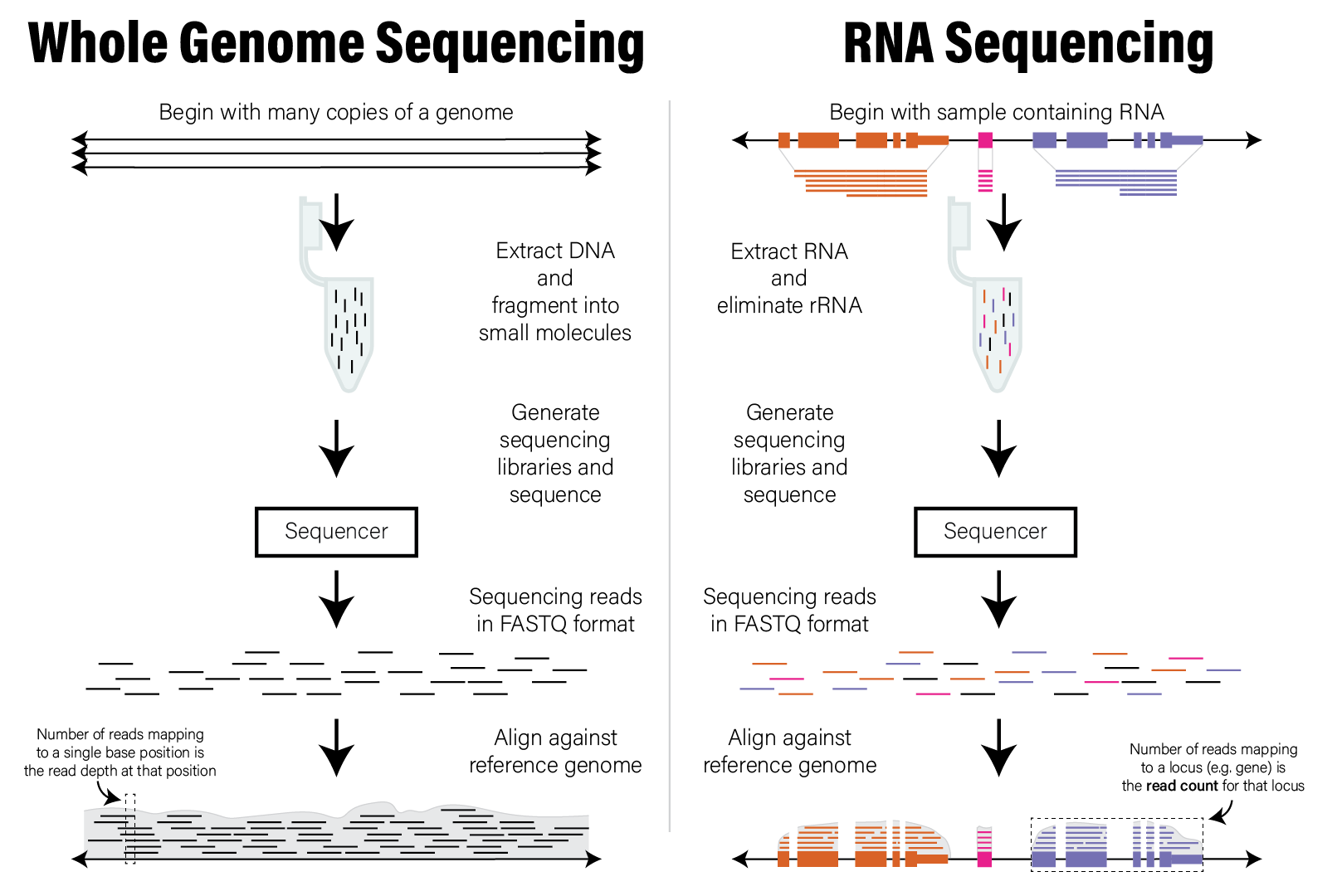
Illustration of WGS and RNASeq read alignment process

8.5.3 Count Data

As mentioned above, the number of reads, or read counts that align to each locus of a genome form a distribution we can use to interpret the data. Count data have two important properties that require special attention:

Count data are integers - the read counts assigned to a particular locus are whole numbers
Counts are non-negative - counts can either be zero or positive; they cannot be negative

These two properties have the important consequence that count data are not normally distributed. Unlike with microarray data, common statistical techniques like linear regression are not directly applicable to count data. We must therefore account for this property of the data prior to statistical analysis in one of two ways:

Use statistical methods that model counts data - generalized linear models that model data using Poisson and Negative Binomial distributions
Transform the data to have be normally distributed - certain statistical transformations, such as regularized log or rank transformations can make counts data more closely follow a normal distribution

We will discuss these strategies in greater detail in the RNASeq Gene Expression Data section.