7.9 Network visualization

The most commonly used package to visualize network is igraph.

library(igraph)

First, let’s create a graph with 15 nodes.

names <- c("Opal", "Tourmaline", "Emerald", "Citrine", "Jasper", "Moonstone", "Agate", "Chalcedony", "Crystal", "Obsidian", "Quartz", "Topaz", "Beryl", "Sugilite", "Sapphire")

Use sample_gnm() to generate a random graph.

set.seed(10)
samp_g <- sample_gnm(
  n = 15, # number of vertices
  m = 20, # total number of edges
  directed = FALSE # if it's a directed network
)

To assign color to vertices, use vertex_attr(). gorder() returns the number of vertices.

vertex_attr(samp_g) <- list(name = names, color = rep("slategray1", gorder(samp_g)))

To assign color to edges, use vertex_attr(). gsize() returns the total number of edges. Here I am assigning random colors.

edge_attr(samp_g) <- list(color = sample(
  x = c("slateblue1", "lightpink1", "steelblue1", "palegreen3"),
  size = gsize(samp_g), replace = TRUE
))

In real case, when you want to modify the color of a specific edge, you need to first find which edge you want to modify…

edges(samp_g)

## [[1]]
## IGRAPH 7328255 UN-- 15 20 -- Erdos renyi (gnm) graph
## + attr: name (g/c), type (g/c), loops (g/l), m (g/n), name (v/c), color
## | (v/c), color (e/c)
## + edges from 7328255 (vertex names):
##  [1] Emerald   --Citrine    Citrine   --Jasper     Tourmaline--Moonstone 
##  [4] Emerald   --Chalcedony Emerald   --Crystal    Opal      --Obsidian  
##  [7] Agate     --Obsidian   Opal      --Quartz     Jasper    --Quartz    
## [10] Agate     --Quartz     Obsidian  --Quartz     Obsidian  --Topaz     
## [13] Tourmaline--Beryl      Agate     --Beryl      Quartz    --Beryl     
## [16] Quartz    --Sugilite   Emerald   --Sapphire   Moonstone --Sapphire  
## [19] Agate     --Sapphire   Sugilite  --Sapphire  
## 
## attr(,"class")
## [1] "igraph.edge"

Then modify it. For example, modify the 1st edge, which is “Emerald–Citrine.”

edge_attr(samp_g, name = "color")[1] <- "red"

To visualize the network, just use plot()!

plot(samp_g)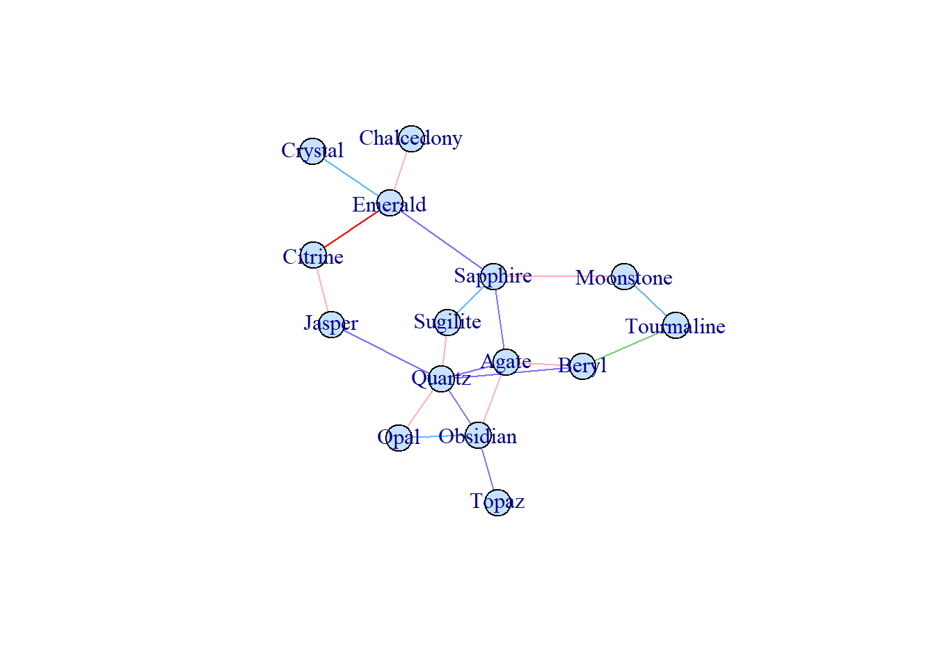

In real-world, we don’t want a random network. Now let’s create our network from scratch.

There are many different ways to create a network. One of the most basic (and easy) ways is using graph_from_data_frame() function in igraph.
1. Create 2 columns in the data frame: from and to. Each row represents an edge, and the entries are vertex names. For instance, as indicated in row 1 below, there is an edge “from Crystal to Moonstone.” In an undirected graph, you can put the two vertices in either way.
2. (optional) Add another column color to represent the color to plot the edge.
3. (optional) You can also add additional information for each edge. For example, add a column weight to specify the weight of this edge. The weight will become useful when you do network analysis later, for example, find the shortest path between two vertices. You can also add other attributes you want, like the “connection_type” here.

set.seed(4)
my_gem_df <- data.frame(
  "from" = c("Crystal", "Crystal", "Crystal", "Crystal", "Topaz", "Obsidian", "Agate", "Topaz"),
  "to" = c("Moonstone", "Citrine", "Obsidian", "Agate", "Citrine", "Topaz", "Moonstone", "Moonstone"),
  "color" = c("slateblue1", "slateblue1", "slateblue1", "steelblue1", "palegreen3", "steelblue1", "lightpink1", "palegreen3"),
  "connection_type" = c(rep(1, 6), 2, 2)
)
my_gem_df$weight <- as.numeric(as.factor(my_gem_df$color))
my_gem_df

##       from        to      color connection_type weight
## 1  Crystal Moonstone slateblue1               1      3
## 2  Crystal   Citrine slateblue1               1      3
## 3  Crystal  Obsidian slateblue1               1      3
## 4  Crystal     Agate steelblue1               1      4
## 5    Topaz   Citrine palegreen3               1      2
## 6 Obsidian     Topaz steelblue1               1      4
## 7    Agate Moonstone lightpink1               2      1
## 8    Topaz Moonstone palegreen3               2      2

Now create an igraph object from the data frame, and assign vertex color.

g <- graph_from_data_frame(my_gem_df, directed = FALSE)
vertex_attr(g) <- list(
  name = c("Crystal", "Topaz", "Obsidian", "Agate", "Moonstone", "Citrine"),
  color = c("slategray1", "slategray1", "slategray1", "lightpink", "slategray1", "lightpink")
)

Again, simply use plot(g) to plot the network. We can also do some fancy customization to play around with the labels! (Remember the connection_type I specified above in the data frame? In edge.lty, 1 is a solid line, and 2 is a dash line)

set.seed(4)
plot(g,
  edge.width = 1.5,
  edge.lty = edge_attr(g, "connection_type"),
  vertex.label.family = "Trebuchet MS",
  vertex.label.font = 3,
  vertex.label.cex = 1,
  vertex.label.dist = 2,
  vertex.label.degree = pi / 2
)

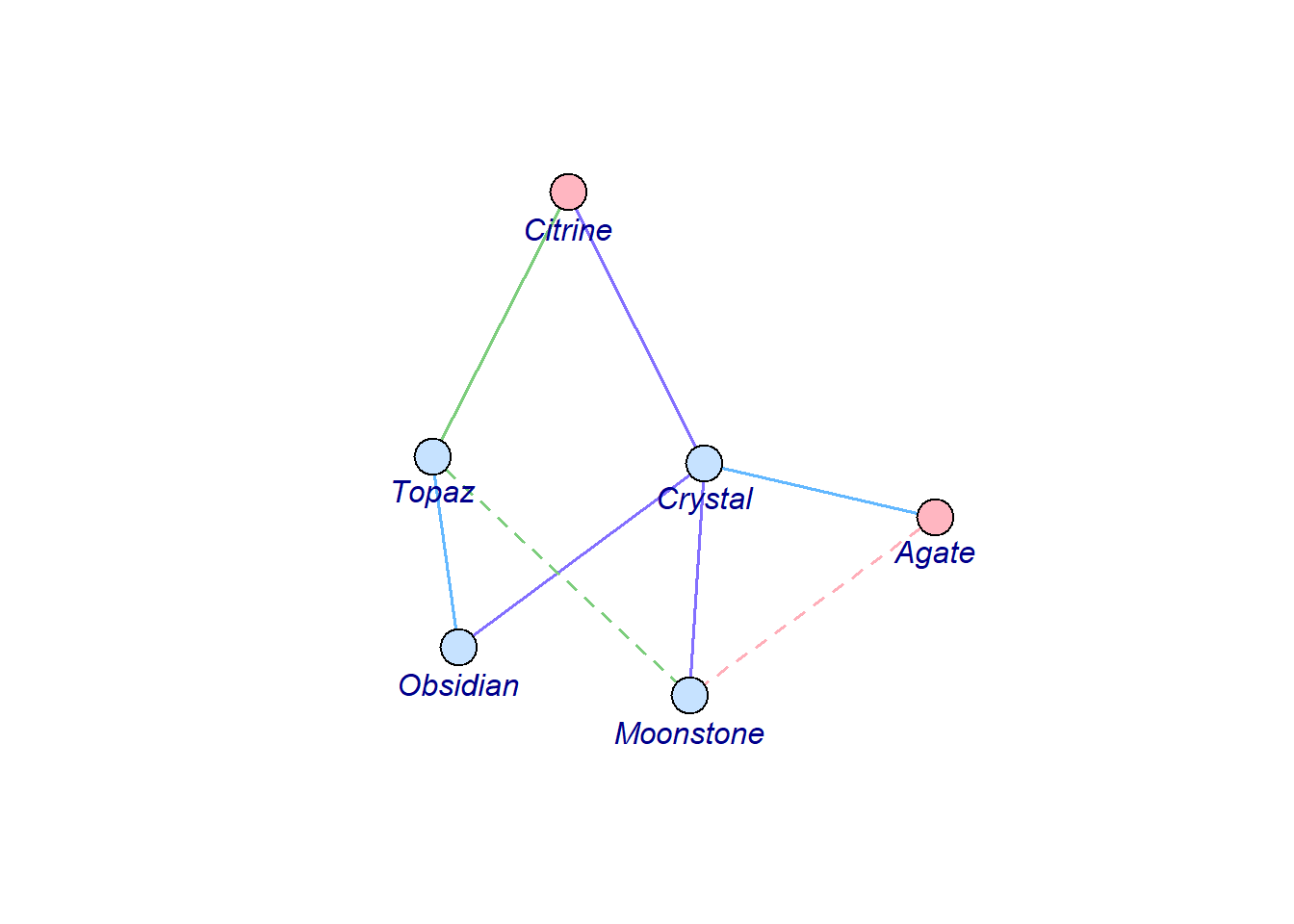
To see the whole list of available arguments available when plotting your network, visit igraph plot manual.

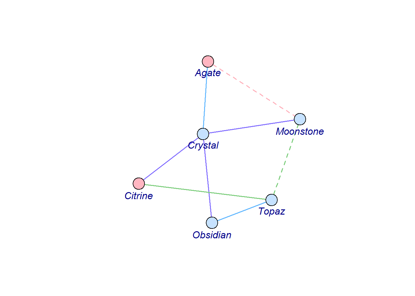
In the case of an directed graph, simply put directed = TRUE when creating the igraph object, and you will see the cute arrows.

g <- graph_from_data_frame(my_gem_df, directed = TRUE)
vertex_attr(g) <- list(
  name = c("Crystal", "Topaz", "Obsidian", "Agate", "Moonstone", "Citrine"),
  color = c("slategray1", "slategray1", "slategray1", "lightpink", "slategray1", "lightpink")
)
set.seed(4)
plot(g,
  edge.width = 1.5,
  edge.lty = edge_attr(g, "connection_type"),
  edge.arrow.size = 0.8,
  vertex.label.family = "Trebuchet MS",
  vertex.label.font = 3,
  vertex.label.cex = 1,
  vertex.label.dist = 2,
  vertex.label.degree = pi / 2
)