5.7.1 dplyr::mutate() - Create new columns using other columns

Many biological analysis procedures perform some kind of statistical test on a collection of features (e.g. genes) and produce p-values that indicate how “surprising” each feature is according to the test. The p-values in our tibble are nominal, i.e. they have not been adjusted for multiple hypotheses. Briefly, when we run multiple tests like we are on each of our three genes, there is a chance that some of the tests will have a small p-value simply by chance. Multiple testing correction procedures adjust nominal p-values to account for this possibility in a number of different ways, but the most common procedure in biological analysis is the Benjamini-Hochberg or False Discovery Rate (FDR) procedure. In R, the p.adjust function can perform several of these procedures, including FDR:

dplyr::mutate(gene_stats,
  test1_padj=p.adjust(test1_p,method="fdr")
)

## # A tibble: 3 x 6
##   gene  test1_stat      test1_p test2_stat  test2_p   test1_padj
##   <chr>      <dbl>        <dbl>      <dbl>    <dbl>        <dbl>
## 1 apoe       12.5  0.103            34.2   0.000013 0.155       
## 2 hoxd1       4.40 0.632            16.3   0.0421   0.632       
## 3 snca       45.7  0.0000000042      0.757 0.915    0.0000000126

Notice how the adjusted p-values are larger than the nominal ones; this is the effect of the multiple testing procedure. Since we have two sets of p-values, we must compute the FDR on each of them, which we can do in the same call to mutate():

gene_stats_mutated <- dplyr::mutate(gene_stats,
  test1_padj=p.adjust(test1_p,method="fdr"),
  test2_padj=p.adjust(test2_p,method="fdr")
)
gene_stats_mutated

## # A tibble: 3 x 7
##   gene  test1_stat      test1_p test2_stat  test2_p   test1_padj test2_padj
##   <chr>      <dbl>        <dbl>      <dbl>    <dbl>        <dbl>      <dbl>
## 1 apoe       12.5  0.103            34.2   0.000013 0.155          0.000039
## 2 hoxd1       4.40 0.632            16.3   0.0421   0.632          0.0632  
## 3 snca       45.7  0.0000000042      0.757 0.915    0.0000000126   0.915

Another common operation is to create new columns derived from the values in multiple other columns. We (or our wetlab colleagues) might decide it is convenient to have a new column with TRUE or FALSE based on whether the gene was significant in either test. Such a column would make it easy to filter genes down to just ones that might be interesting in tools like Excel. We can create new columns from multiple columns just as easily using the mutate() function:

dplyr::mutate(gene_stats_mutated,
  signif_either=(test1_padj < 0.05 | test2_padj < 0.05),
  signif_both=(test1_padj < 0.05 & test2_padj < 0.05)
)

## # A tibble: 3 x 9
##   gene  test1_stat      test1_p test2_stat  test2_p   test1_padj test2_padj
##   <chr>      <dbl>        <dbl>      <dbl>    <dbl>        <dbl>      <dbl>
## 1 apoe       12.5  0.103            34.2   0.000013 0.155          0.000039
## 2 hoxd1       4.40 0.632            16.3   0.0421   0.632          0.0632  
## 3 snca       45.7  0.0000000042      0.757 0.915    0.0000000126   0.915   
## # ... with 2 more variables: signif_either <lgl>, signif_both <lgl>

Recall that the | and & operators execute ‘or’ and ‘and’ logic, respectively. The above example required the creation of a new variable gene_stats_mutated because the columns test1_padj and test2_padj need to be in the tibble before computing the new fields. However, in mutate(), columns created first in the function call are available to later columns. In the following example, note that test1_padj is created first and then used to create the signif columns:

dplyr::mutate(gene_stats,
  test1_padj=p.adjust(test1_p,method="fdr"), # test1_padj created
  test2_padj=p.adjust(test2_p,method="fdr"),
  signif_either=(test1_padj < 0.05 | test2_padj < 0.05), #test1_padj used
  signif_both=(test1_padj < 0.05 & test2_padj < 0.05)
)

## # A tibble: 3 x 9
##   gene  test1_stat      test1_p test2_stat  test2_p   test1_padj test2_padj
##   <chr>      <dbl>        <dbl>      <dbl>    <dbl>        <dbl>      <dbl>
## 1 apoe       12.5  0.103            34.2   0.000013 0.155          0.000039
## 2 hoxd1       4.40 0.632            16.3   0.0421   0.632          0.0632  
## 3 snca       45.7  0.0000000042      0.757 0.915    0.0000000126   0.915   
## # ... with 2 more variables: signif_either <lgl>, signif_both <lgl>

The alternative would be to split this into two mutate() commands, the first creating the adjusted p-value columns and the second creating the significance columns. dplyr recognizes how common it is to build new variables off of other new variables in a mutate() command, and therefore provides this convenient behavior.

mutate() can also be used to modify columns in place. The official convention for human gene symbols is that they are upper case, but for some reason our tibble contains lower case gene symbols. We can correct this using mutate() but first we should talk about the stringr package which makes working with strings much easier than with base R functions.

5.7.2 stringr - Working with character values

Base R does not have very convenient functions for working with character strings (or just strings). This is due to its original intent a statistical programming language, where string manipulation is not (in principle) a common operation. However, in practice, we must frequently manipulate strings while loading, cleaning, and analyzing datasets. The stringr package aims to make working with strings “as easy as possible.”

The package includes many useful functions for operating on strings, including searching for patterns, mutating strings, lexicographical sorting, combining multiple strings together (i.e. concatenation), and performing complex search/replace operations. There are far too many useful functions to cover here and you should become comfortable reading the stringr documentation and the very helpful stringr cheatsheet.

In the previous section, we noted that the gene symbols in our tibble were lower case while official gene symbols are in upper case. We can use the stringr function stringr::str_to_upper() with the dplyr::mutate() function to perform this adjustment easily:

dplyr::mutate(gene_stats,
  gene=stringr::str_to_upper(gene)
)

## # A tibble: 3 x 5
##   gene  test1_stat      test1_p test2_stat  test2_p
##   <chr>      <dbl>        <dbl>      <dbl>    <dbl>
## 1 APOE       12.5  0.103            34.2   0.000013
## 2 HOXD1       4.40 0.632            16.3   0.0421  
## 3 SNCA       45.7  0.0000000042      0.757 0.915

Now are gene symbols have the appropriate case, and our wetlab colleagues won’t complain about it. :)

5.7.2.1 Regular expressions

Many of the string operations in the stringr package use regular expression syntax. A regular expression is a sequence of characters that describes patterns in text. Regular expressions are written in a sort of mini programming language where certain characters have special meaning that help in defining search patterns that identifies the location of sequences of characters in text that follow a particular pattern specified by the regular expression. This is similar to the “Find” functionality in many word processors, but is more powerful due to the flexibility of the patterns that can be found.

A simple example will be helpful. Let’s say we have a tibble containing the result of a (made-up) statistical test for all the genes in a genome:

de_genes

## # A tibble: 39,535 x 4
##    hgnc_symbol  mean        p    padj
##    <chr>       <int>    <dbl>   <dbl>
##  1 MT-TF        5799 0.000910 0.00941
##  2 MT-RNR1       153 0.0272   0.0342 
##  3 MT-TV         115 0.0228   0.0301 
##  4 MT-RNR2       495 0.00318  0.0123 
##  5 MT-TL1      20201 0.000377 0.00841
##  6 MT-ND1        160 0.0179   0.0258 
##  7 MT-TI        3511 0.00247  0.0115 
##  8 MT-TQ         772 0.00376  0.0129 
##  9 MT-TM         301 0.00325  0.0124 
## 10 MT-ND2         12 0.107    0.111  
## # ... with 39,525 more rows

Now let’s say we’re interested in examining the results for the BRCA family of genes, BRCA1 and BRCA2. We can use filter() on the data frame to look for them individually:

de_genes %>% filter(hgnc_symbol == "BRCA1" | hgnc_symbol == "BRCA2")

## # A tibble: 2 x 4
##   hgnc_symbol  mean      p   padj
##   <chr>       <int>  <dbl>  <dbl>
## 1 BRCA1          41 0.0321 0.0386
## 2 BRCA2         447 0.0140 0.0223

This isn’t so bad, but we can do the same thing with stringr::str_detect() , which returns TRUE if the provided pattern matches the input and FALSE otherwise, a regular expression, and the [dplyr::filter() function], which is described in greater detail in a later section:

dplyr::filter(de_genes, str_detect(hgnc_symbol,"^BRCA[12]$"))

## # A tibble: 2 x 4
##   hgnc_symbol  mean      p   padj
##   <chr>       <int>  <dbl>  <dbl>
## 1 BRCA1          41 0.0321 0.0386
## 2 BRCA2         447 0.0140 0.0223

The argument "^BRCA[12]$" is a regular expression that searches for the following:

• Search for genes that start with the characters BRCA - the ^ at the beginning of the pattern stands for the start of the string
• For genes that start with BRCA, then look for genes where the next character is either 1 or 2 with [12] - the characters between the [] are searched for explicitly, and any character encountered that is not listed between them results in a non-match
• For genes that start with BRCA followed with either a 1 or a 2, match successfully if the number is at the end of the name - the $ at the end of the pattern stands for the end of the string

We can use these principles to find genes with more complex naming conventions. The Homeobox (HOX) genes encode DNA binding proteins that regulate gene expression of genes involved in morphgenesis and cell differentiation in vertebrates. In humans, HOX genes are organized into 4 clusters of paralogs that were the result of three DNA duplication events in the distant evolutionary past(Abbasi 2015), where each cluster encodes a subset of 13 distinct HOX genes placed next to each other. Each of these clusters has been assigned a letter identifier A-D (e.g. HOXA, HOXB, HOXC, and HOXD) and each paralogous gene within each cluster is assigned the same number (e.g. HOXA4, HOXB4, HOXC4, and HOXD4 are paralogs). There are 13 HOX genes in total, though not all genes remain in all clusters (e.g. HOXA1, HOXB1, and HOXD1 exist but HOXC1 was lost over time). The following figure depicts the human HOX gene clusters:

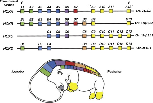
Human HOX gene clusters - Veraksa, A.; Del Campo, M.; McGinnis, W. Developmental Patterning Genes and their Conserved Functions: From Model Organisms to Humans. Mol. Genet. Metab. 2000, 69 (2), 85–100.

Let’s say we want to extract out all the HOX genes from our gene statistics. We can write a regular expression that matches the pattern described above:

dplyr::filter(de_genes, str_detect(hgnc_symbol,"^HOX[A-D][0-9]+$")) %>%
  dplyr::arrange(hgnc_symbol)

## # A tibble: 39 x 4
##    hgnc_symbol  mean        p    padj
##    <chr>       <int>    <dbl>   <dbl>
##  1 HOXA1        8734 0.000858 0.00934
##  2 HOXA10       4149 0.00152  0.0102 
##  3 HOXA11        567 0.0101   0.0188 
##  4 HOXA13        411 0.0105   0.0191 
##  5 HOXA2         554 0.00600  0.0151 
##  6 HOXA3          18 0.0919   0.0959 
##  7 HOXA4         475 0.0113   0.0199 
##  8 HOXA5         434 0.0127   0.0211 
##  9 HOXA6        3983 0.00252  0.0115 
## 10 HOXA7         897 0.00961  0.0183 
## # ... with 29 more rows

In this query we used two new regular expression features:

• within the [] we specified a range of characters A-D and 0-9 which will match any of the characters between A and D (i.e. A, B, C, or D) and 0 and 9 respectively
• the + character means “match one or more of the preceding expression,” which in our case is the [0-9]. This allows us to match genes with only a single number (e.g. HOXA1) as well as double digit numbers (e.g. HOXA10).

Since we know the cluster identifier part of the HOX gene names (i.e. the [A-D] part) is exactly one character long, we could alternatively write the regular expression as follows, using the special . character:

dplyr::filter(de_genes, str_detect(hgnc_symbol,"^HOX.[0-9]+$")) %>%
  dplyr::arrange(hgnc_symbol)

## # A tibble: 39 x 4
##    hgnc_symbol  mean        p    padj
##    <chr>       <int>    <dbl>   <dbl>
##  1 HOXA1        8734 0.000858 0.00934
##  2 HOXA10       4149 0.00152  0.0102 
##  3 HOXA11        567 0.0101   0.0188 
##  4 HOXA13        411 0.0105   0.0191 
##  5 HOXA2         554 0.00600  0.0151 
##  6 HOXA3          18 0.0919   0.0959 
##  7 HOXA4         475 0.0113   0.0199 
##  8 HOXA5         434 0.0127   0.0211 
##  9 HOXA6        3983 0.00252  0.0115 
## 10 HOXA7         897 0.00961  0.0183 
## # ... with 29 more rows

Here, the . character is interpreted by the regex to match any single character, regardless of what it is, between the HOX part and the number part. This also requires that there exist exactly one character between the two parts; a gene symbol HOX1 would not be matched, because the 1 would match to the ., but no number remains to match to the [0-9]+ part.

Sometimes you want to search text for characters that are considered special in the regular expression language. For example, if you had a list of filenames:

filenames <- tribble(
  ~name,
  "annotation.csv",
  "file1.txt",
  "file2.txt",
  "results.csv"
)

and wanted to limit to just those with the .txt extension, you need to match using a literal . character:

filter(filenames, stringr::str_detect(name,"[.]txt$"))

## # A tibble: 2 x 1
##   name     
##   <chr>    
## 1 file1.txt
## 2 file2.txt

Inside a [], characters do not have their usual regular expression meaning, and therefore [.] will match a literal . character. Instead of using the [] syntax, you may also escape these literal characters using two back slashes:

filter(filenames, stringr::str_detect(name,"\\.txt$"))

## # A tibble: 2 x 1
##   name     
##   <chr>    
## 1 file1.txt
## 2 file2.txt

Regular expressions are very powerful, and can do much more than what is described here. See the regular expression tutorial linked in the readmore box to learn more details.

• R for Data Science - Strings
• stringr documentation
• stringr cheatsheet
• RegexOne - regular expression tutorial

5.7.3 dplyr::select() - Subset Columns by Name

Our mutate() operations above created a number of new columns in our tibble, but we did not specify where in the tibble the new columns should go. Let’s consider the mutated tibble we created with all four new columns:

dplyr::mutate(gene_stats,
  test1_padj=p.adjust(test1_p,method="fdr"),
  test2_padj=p.adjust(test2_p,method="fdr"),
  signif_either=(test1_padj < 0.05 | test2_padj < 0.05),
  signif_both=(test1_padj < 0.05 & test2_padj < 0.05),
  gene=stringr::str_to_upper(gene)
)

## # A tibble: 3 x 9
##   gene  test1_stat      test1_p test2_stat  test2_p   test1_padj test2_padj
##   <chr>      <dbl>        <dbl>      <dbl>    <dbl>        <dbl>      <dbl>
## 1 APOE       12.5  0.103            34.2   0.000013 0.155          0.000039
## 2 HOXD1       4.40 0.632            16.3   0.0421   0.632          0.0632  
## 3 SNCA       45.7  0.0000000042      0.757 0.915    0.0000000126   0.915   
## # ... with 2 more variables: signif_either <lgl>, signif_both <lgl>

From a readability standpoint, it might be helpful if all the columns that are about each test were grouped together, rather than having to look at the end of the tibble to find them.

The dplyr::select() function allows you to pick specific columns out of a larger tibble in whatever order you choose:

stats <- dplyr::select(gene_stats, test1_stat, test2_stat)
stats

## # A tibble: 3 x 2
##   test1_stat test2_stat
##        <dbl>      <dbl>
## 1      12.5      34.2  
## 2       4.40     16.3  
## 3      45.7       0.757

Here we have explicitly selected the statistics columns. dplyr also has helper functions that allow for more flexible selection of columns. For example, if all of the columns we wished to select ended with _stat, we could use the ends_with() helper function:

stats <- dplyr::select(gene_stats, ends_with("_stat"))
stats

## # A tibble: 3 x 2
##   test1_stat test2_stat
##        <dbl>      <dbl>
## 1      12.5      34.2  
## 2       4.40     16.3  
## 3      45.7       0.757

If you so desire, select() allows for the renaming of selected columns:

stats <- dplyr::select(gene_stats,
  t=test1_stat,
  chisq=test2_stat
)
stats

## # A tibble: 3 x 2
##       t  chisq
##   <dbl>  <dbl>
## 1 12.5  34.2  
## 2  4.40 16.3  
## 3 45.7   0.757

If we knew that these test statistics actually corresponded to some kind of t-test and a \(\chi\)-squared test, naming the columns of the tibble appropriately may help others (and possibly you) understand your code better.

We can use the dplyr::select() function to obtain our desired column order:

dplyr::mutate(gene_stats,
  test1_padj=p.adjust(test1_p,method="fdr"),
  test2_padj=p.adjust(test2_p,method="fdr"),
  signif_either=(test1_padj < 0.05 | test2_padj < 0.05),
  signif_both=(test1_padj < 0.05 & test2_padj < 0.05),
  gene=stringr::str_to_upper(gene)
) %>%
dplyr::select(
    gene,
    test1_stat, test1_p, test1_padj,
    test2_stat, test2_p, test2_padj,
    signif_either,
    signif_both
)

## # A tibble: 3 x 9
##   gene  test1_stat      test1_p   test1_padj test2_stat  test2_p test2_padj
##   <chr>      <dbl>        <dbl>        <dbl>      <dbl>    <dbl>      <dbl>
## 1 APOE       12.5  0.103        0.155            34.2   0.000013   0.000039
## 2 HOXD1       4.40 0.632        0.632            16.3   0.0421     0.0632  
## 3 SNCA       45.7  0.0000000042 0.0000000126      0.757 0.915      0.915   
## # ... with 2 more variables: signif_either <lgl>, signif_both <lgl>

Now the order of our columns is clear and convenient. It is not necessary to list the columns for each test statistic on the same line, but the author thinks this makes the code easier to read and understand.

5.7.4 dplyr::filter() - Pick rows out of a data set

Often, the first step in interpreting an analysis is to identify the features that are significant at some adjusted p-value threshold. First we will save our mutated tibble to another variable, to aid in demonstration:

gene_stats_mutated <- dplyr::mutate(gene_stats,
  test1_padj=p.adjust(test1_p,method="fdr"),
  test2_padj=p.adjust(test2_p,method="fdr"),
  signif_either=(test1_padj < 0.05 | test2_padj < 0.05),
  signif_both=(test1_padj < 0.05 & test2_padj < 0.05),
  gene=stringr::str_to_upper(gene)
) %>%
dplyr::select(
    gene,
    test1_stat, test1_p, test1_padj,
    test2_stat, test2_p, test2_padj,
    signif_either,
    signif_both
)

Now we can use the dplyr::filter() function to select rows based on whether they are significant in either test this with our above example.

dplyr::filter(gene_stats_mutated, test1_padj < 0.05)

## # A tibble: 1 x 9
##   gene  test1_stat      test1_p   test1_padj test2_stat test2_p test2_padj
##   <chr>      <dbl>        <dbl>        <dbl>      <dbl>   <dbl>      <dbl>
## 1 SNCA        45.7 0.0000000042 0.0000000126      0.757   0.915      0.915
## # ... with 2 more variables: signif_either <lgl>, signif_both <lgl>

dplyr::filter(gene_stats_mutated, test2_padj < 0.05)

## # A tibble: 1 x 9
##   gene  test1_stat test1_p test1_padj test2_stat  test2_p test2_padj
##   <chr>      <dbl>   <dbl>      <dbl>      <dbl>    <dbl>      <dbl>
## 1 APOE        12.5   0.103      0.155       34.2 0.000013   0.000039
## # ... with 2 more variables: signif_either <lgl>, signif_both <lgl>

Here we are filtering the result so that only genes with nominal p-value less than 0.05 remain. Note we filter on the two tests separately, but we can also combine these tests using logical operators to achieve different results:

# | means "logical or", meaning the row is retained if either condition is true
dplyr::filter(gene_stats_mutated, test1_padj < 0.05 | test2_padj < 0.05)

## # A tibble: 2 x 9
##   gene  test1_stat      test1_p   test1_padj test2_stat  test2_p test2_padj
##   <chr>      <dbl>        <dbl>        <dbl>      <dbl>    <dbl>      <dbl>
## 1 APOE        12.5 0.103        0.155            34.2   0.000013   0.000039
## 2 SNCA        45.7 0.0000000042 0.0000000126      0.757 0.915      0.915   
## # ... with 2 more variables: signif_either <lgl>, signif_both <lgl>

Only APOE and SCNA are significant in at least one of the tests.

# & means "logical and", meaning the row is retained only if both conditions are true
dplyr::filter(gene_stats_mutated, test1_padj < 0.05 & test2_padj < 0.05)

## # A tibble: 0 x 9
## # ... with 9 variables: gene <chr>, test1_stat <dbl>, test1_p <dbl>,
## #   test1_padj <dbl>, test2_stat <dbl>, test2_p <dbl>, test2_padj <dbl>,
## #   signif_either <lgl>, signif_both <lgl>

It looks like we don’t have any genes that are significant by both tests. Filtering results like this is one of the most common operations we do on the results of biological analyses.

5.7.5 dplyr::arrange() - Order rows based on their values

Another common operation when working with biological analysis results is ordering them by some meaningful value. Like above, p-values are often used to prioritize results by simply sorting them in ascending order. The arrange() function is how to perform this sorting in tidyverse:

stats_sorted_by_test1_p <- dplyr::arrange(gene_stats, test1_p)
stats_sorted_by_test1_p

## # A tibble: 3 x 5
##   gene  test1_stat      test1_p test2_stat  test2_p
##   <chr>      <dbl>        <dbl>      <dbl>    <dbl>
## 1 snca       45.7  0.0000000042      0.757 0.915   
## 2 apoe       12.5  0.103            34.2   0.000013
## 3 hoxd1       4.40 0.632            16.3   0.0421

In general, the larger the magnitude of the statistic, the smaller the p-value (for two-tailed tests), so if we so desired we could induce a similar ranking by arranging the data by the statistic in descending order:

# desc() is a helper function that causes the results to be sorted in descending
# order for the given column
dplyr::arrange(gene_stats, desc(abs(test1_stat)))

## # A tibble: 3 x 5
##   gene  test1_stat      test1_p test2_stat  test2_p
##   <chr>      <dbl>        <dbl>      <dbl>    <dbl>
## 1 snca       45.7  0.0000000042      0.757 0.915   
## 2 apoe       12.5  0.103            34.2   0.000013
## 3 hoxd1       4.40 0.632            16.3   0.0421

Here we first apply the base R abs() function to compute the absolute value of the test 1 statistic and then specify that we want to sort largest first. Note although we don’t have any negative values in our dataset, we should not assume that in general, so it is safer for us to be complete and add the absolute value call in case later we decide to copy and paste this code into another analysis. That’s pretty much all there is to arrange().

5.7.6 Putting it all together

In the previous sections, we performed the following operations:

1. Created new columns by computing false discovery rate on the nominal p-values using the dplyr::mutate() and p.adjust functions
2. Created new columns that indicate the patterns of significance for each gene using dplyr::mutate()
3. Mutated the gene symbol case using stringr::str_to_upper and dplyr::mutate()
4. Reordered the columns to group related variables with select()
5. Filtered genes based on whether they have an adjusted p-value less than 0.05 for either and both statistical tests using dplyr::filter()
6. Sorted the results by p-value using dplyr::arrange()

For the sake of illustration, these steps were presented separately, but together they represent a single unit of data processing and thus might profitably be done in the same R command using %>%:

gene_stats <- dplyr::mutate(gene_stats,
  test1_padj=p.adjust(test1_p,method="fdr"),
  test2_padj=p.adjust(test2_p,method="fdr"),
  signif_either=(test1_padj < 0.05 | test2_padj < 0.05),
  signif_both=(test1_padj < 0.05 & test2_padj < 0.05),
  gene=stringr::str_to_upper(gene)
) %>%
dplyr::select(
    gene,
    test1_stat, test1_p, test1_padj,
    test2_stat, test2_p, test2_padj,
    signif_either,
    signif_both
) %>%
dplyr::filter(
  test1_padj < 0.05 | test2_padj < 0.05
) %>%
dplyr::arrange(
  test1_p
)
gene_stats

## # A tibble: 2 x 9
##   gene  test1_stat      test1_p   test1_padj test2_stat  test2_p test2_padj
##   <chr>      <dbl>        <dbl>        <dbl>      <dbl>    <dbl>      <dbl>
## 1 SNCA        45.7 0.0000000042 0.0000000126      0.757 0.915      0.915   
## 2 APOE        12.5 0.103        0.155            34.2   0.000013   0.000039
## # ... with 2 more variables: signif_either <lgl>, signif_both <lgl>

This complete pipeline now contains all of our manipulations and our mutated tibble can be passed on to downstream analysis or collaborators.