8.2.1 Types of Biological Data

In very general terms, there are five types of data used in biological data analysis: raw/primary data, processed data, analysis results, metadata, and annotation data.

Raw/primary data. These data are the primary observations made by whatever instruments/techniques we are using for our experiment. These may include high-throughput sequencing data, mass/charge ratio data from mass spectrometry, 16S rRNA sequencing data from metagenomic studies, SNPs from genotyping assays, etc. These data can be very large and are often not efficiently processed using R. Instead, specialized tools built outside of R are used to first process the primary data into a form that is amenable to analysis. The most common primary biological data types include Microarrays, High Throughput Sequencing data, and mass spectrometry data.

Processed data. Processed data is the result of any analysis or transformation of primary data into an intermediate, more interpretable form. For example, when performing gene expression analysis with RNASeq, short reads that form the primary data are typically aligned against a genome and then counted against annotated genes, resulting in a count for each gene in the genome. Typically, these counts are then combined for many samples into a single matrix and subject to downstream analyses like differential expression.

Analysis results. Analysis results aren’t data per se, but are the results of analysis of primary data or processed results. For example, in gene expression studies, a first analysis is often differential expression, where each gene in the genome is tested for expression associated with some outcome of interest across many samples. Each gene then has a number of statistics and related values, like log2 fold change, nominal and adjusted p-value, etc. These forms of data are usually what we use to form interpretations of our datasets and therefore we must manipulate them in much the same way as any other dataset.

Metadata. In most experimental settings, multiple samples have been processed and had the same primary data type collected. These samples also have information associated with them, which is here termed metadata, or “data about data.” In our gene expression of post mortem brain experiments mentioned above, the information about the individuals themselves, including age at death, whether the person had a disease, the measurements of tissue quality, etc. is the metadata. The primary and processed data and metadata are usually stored in different files, where the metadata (or sample information or sample data, etc) will have one column indicating the unique identifier (ID) of each sample. The processed data will typically have columns named for each of the sample IDs.

Annotation data. A tremendous amount of knowledge has been generated about biological entities, e.g. genes, especially since the publication of the human genome. Annotation data is publicly available information about the features we measure in our experiments. This may come in the form of the coordinates in a genome where genes exist, any known functions of those genes, the domains found in proteins and their relative sequence, gene identifier cross references across different gene naming systems (e.g. symbol vs Ensembl ID), single nucleotide polymorphism genomic locations and associations with traits or diseases, etc. This is information that we use to aid in interpretation of our experimental data but generally do not generate ourselves. Annotation data comes in many forms, some of which are in CSV format.

The figure below contains a simple diagram of how these different types of data work together for a typical biological data analysis.

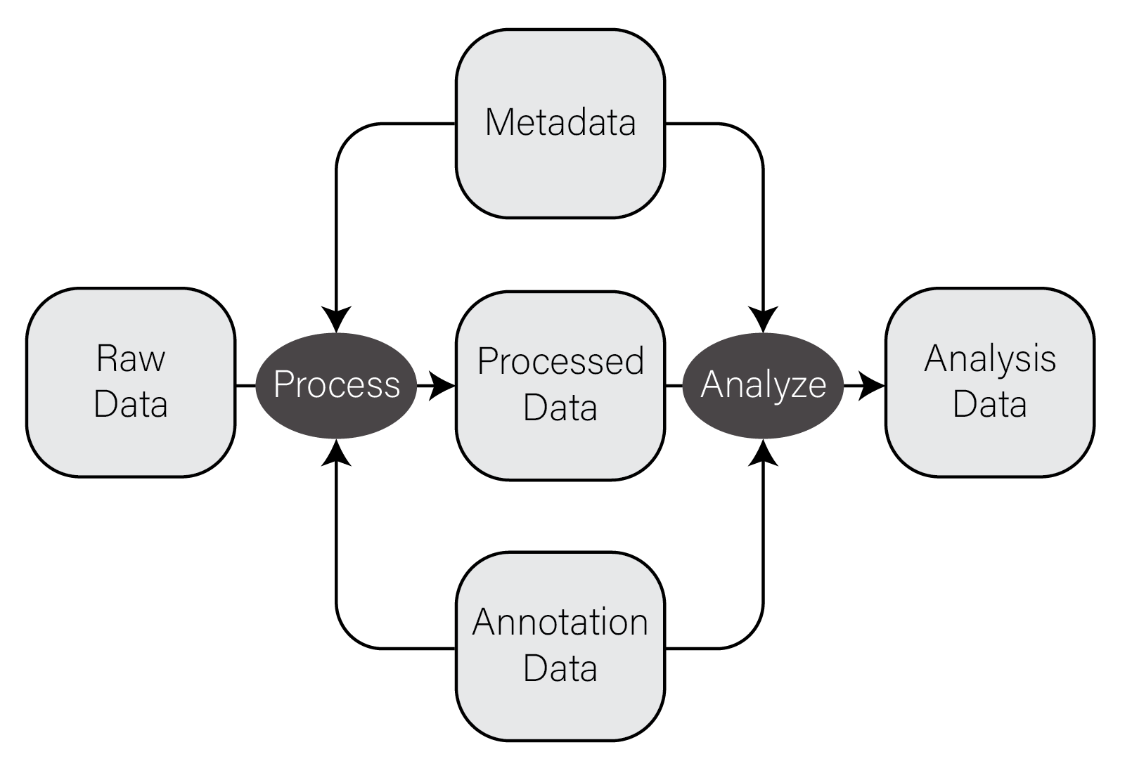
Information flow in biological data analysis

8.2.2 CSV Files

The most common, convenient, and flexible data file format in biology and bioinformatics is the character-delimited or character-separated text file. These files are plain text files (i.e. not the native file format of any specific program, like Excel) that generally contain rectangles of data. When formatted correctly, you can think of these files as containing a grid or matrix of data values with some number of columns, each of which has the same number of values. Each line of these files has some number of data values separated by a consistent character, most commonly the comma which are called comma-separated value, or “CSV,” files and filenames typically end with the extension .csv. Note that other characters, especially the character, may be used to create valid files in this format, and all the same general principles apply. This is an example of a simple CSV file:

id,somevalue,category,genes
1,2.123,A,APOE
4,5.123,B,"HOXA1,HOXB1"
7,8.123,,SNCA

Some properties and principles of CSV files:

• The first line often but not always contains the column names of each column
• Each value is delimited by the same character, in this case ,
• Values can be any value, including numbers and characters
• When a value contains the delimiting character (e.g. HOXA1,HOXB1 contains a ,), the value is wrapped in double quotes
• Values can be missing, indicated by sequential delimiters (i.e. ,, or one , at the end of the line, if the last column value is missing)
• There is no delimiter at the end of the lines
• To be well-formatted every line must have the same number of delimited values

These same properties and principles apply to all character-separated files, regardless of the specific delimiter used. If a file follows these principles, they can be loaded very easily into R or any other data analysis setting. ### Common Biological Data Matrices

Typically the first data set you will work with in R is processed data as described in the previous section. This data has been transformed from primary data in some way such that it (usually) forms a numeric matrix with features as rows and samples as columns. The first column of these files usually contains a feature identifier, e.g. gene identifier, genomic locus, probe set ID, etc and the remaining columns have numerical values, one per sample. The first row is usually column names for all the columns in the file. Below is an example of one of these files from a microarray gene expression dataset loaded into R:

intensities <- read_csv("example_intensity_data.csv")
intensities
# A tibble: 54,675 x 36
   probe     GSM972389 GSM972390 GSM972396 GSM972401 GSM972409 GSM972412 GSM972413 GSM972422 GSM972429
   <chr>         <dbl>     <dbl>     <dbl>     <dbl>     <dbl>     <dbl>     <dbl>     <dbl>     <dbl>
 1 1007_s_at      9.54     10.2       9.72      9.68      9.35      9.89      9.70      9.67      9.87
 2 1053_at        7.62      7.92      7.17      7.24      8.20      6.87      6.62      7.23      7.45
 3 117_at         5.50      5.56      5.06      7.44      5.19      5.72      5.87      6.15      5.46
 4 121_at         7.27      7.96      7.42      7.34      7.49      7.76      7.44      7.66      8.02
 5 1255_g_at      2.79      3.10      2.78      2.91      3.02      2.73      2.78      3.56      2.83
 6 1294_at        7.51      7.28      7.00      7.18      7.38      6.98      6.90      7.54      7.66
 7 1316_at        3.89      4.36      4.24      3.94      4.20      4.34      4.06      4.24      4.11
 8 1320_at        4.65      4.91      4.70      4.78      5.06      4.71      4.55      4.58      5.10
 9 1405_i_at      8.03      7.47      5.42      7.21      9.48      6.79      6.57      8.50      6.36
10 1431_at        3.09      3.78      3.33      3.12      3.21      3.27      3.37      3.84      3.32
# ... with 54,665 more rows, and 26 more variables: GSM972433 <dbl>, GSM972438 <dbl>, GSM972440 <dbl>,
#   GSM972443 <dbl>, GSM972444 <dbl>, GSM972446 <dbl>, GSM972453 <dbl>, GSM972457 <dbl>,
#   GSM972459 <dbl>, GSM972463 <dbl>, GSM972467 <dbl>, GSM972472 <dbl>, GSM972473 <dbl>,
#   GSM972475 <dbl>, GSM972476 <dbl>, GSM972477 <dbl>, GSM972479 <dbl>, GSM972480 <dbl>,
#   GSM972487 <dbl>, GSM972488 <dbl>, GSM972489 <dbl>, GSM972496 <dbl>, GSM972502 <dbl>,
#   GSM972510 <dbl>, GSM972512 <dbl>, GSM972521 <dbl>

The file has 54,676 rows, consisting of one header row which R loads in as the column names, and the remaining are probe sets, one per row. There are 36 columns, where the first contains the probe set ID (e.g. 1007_s_at) and the remaining 35 columns correspond to samples.

8.2.3 Biological data is NOT Tidy!

As mentioned in the tidy data section, the tidyverse packages assume data to be in so-called “tidy format,” with variables as columns and observations as rows. Unfortunately, certain forms of biological data are typically available in the opposite orientation - variables are in rows and observations are in columns. This is primarily true in feature data matrices, e.g. gene expression counts matrices, where the number of variables (e.g. genes) is much larger than the number of samples, which tend to be small very small compared with the number of features. This format is convenient for humans to interact with using, e.g. spreadsheet programs like Microsoft Excel, but can unfortunately make performing certain operations on them challenging in tidyverse.

For example, consider the microarray expression dataset in the previous section. Each of the 54,676 rows is a probeset, and each of the 35 numeric columns is a sample. This is a very large number of probesets to consider, especially if we plan to conduct a statistical test on each, which would impose a substantial multiple hypothesis testing burden on our results. We may therefore wish to eliminate probesets that have very low variance from the overall dataset, since these probesets are not likely to have a detectable statistical difference in our tests. However, computing the variance for each probeset is a computation across all columns, not on columns themselves, and this is not what tidyverse is designed to do well. Said differently, R and tidyverse do not operate by default on the rows of a data frame, tibble, or matrix.

Both base R and tidyverse are optimized to perform computations on columns, not rows. The reasons for this are buried in the details of how the R program itself was written to organize data internally and are beyond the scope of this book. The consequence of this design choice is that, while we can perform operations on the rows rather than the columns of a data structure, our code may perform very poorly (i.e. take a very long time to run).

When working with these datasets, we have a couple options to deal with this issue:

• Pivot into long format. As described in the Rearranging Data section, we can rearrange our tibble to be more amenable to certain computations. In our earlier example, we wish to group all of our measurements by probeset and compute the variance of each, then possibly filter out probesets based on low variance. We can therefore combine pivot_longer(), group_by(), summarize(), and finally left_join() to perform this operation. Exactly how to do this is left as an exercise in Assignment 1.

• Compute row-wise statistics using apply(). As described in Iteration, R is a functional programming language and implements iteration in a functional style using the apply() function. The apply() function accepts a MARGIN argument of 1 or 2 if the provided function is to be applied to the columns or rows, respectively. This method can be used to compute a summary statistic on each row of a tibble and the result saved back into the tibble using the column set operator:

  intensity_variance <- apply(intensities, 2, var)
  intensities$variance <- intensity_variance