- Syllabus
- 1 Introduction
- 2 Data in Biology
- 3 Preliminaries
- 4 R Programming
- 4.1 Before you begin
- 4.2 Introduction
- 4.3 R Syntax Basics
- 4.4 Basic Types of Values
- 4.5 Data Structures
- 4.6 Logical Tests and Comparators
- 4.7 Functions
- 4.8 Iteration
- 4.9 Installing Packages
- 4.10 Saving and Loading R Data
- 4.11 Troubleshooting and Debugging
- 4.12 Coding Style and Conventions
- 4.12.1 Is my code correct?
- 4.12.2 Does my code follow the DRY principle?
- 4.12.3 Did I choose concise but descriptive variable and function names?
- 4.12.4 Did I use indentation and naming conventions consistently throughout my code?
- 4.12.5 Did I write comments, especially when what the code does is not obvious?
- 4.12.6 How easy would it be for someone else to understand my code?
- 4.12.7 Is my code easy to maintain/change?
- 4.12.8 The
stylerpackage
- 5 Data Wrangling
- 6 Data Science
- 7 Data Visualization
- 8 Biology & Bioinformatics
- 8.1 R in Biology
- 8.2 Biological Data Overview
- 8.3 Bioconductor
- 8.4 Microarrays
- 8.5 High Throughput Sequencing
- 8.6 Gene Identifiers
- 8.7 Gene Expression
- 8.7.1 Gene Expression Data in Bioconductor
- 8.7.2 Differential Expression Analysis
- 8.7.3 Microarray Gene Expression Data
- 8.7.4 Differential Expression: Microarrays (limma)
- 8.7.5 RNASeq
- 8.7.6 RNASeq Gene Expression Data
- 8.7.7 Filtering Counts
- 8.7.8 Count Distributions
- 8.7.9 Differential Expression: RNASeq
- 8.8 Gene Set Enrichment Analysis
- 8.9 Biological Networks .
- 9 EngineeRing
- 10 RShiny
- 11 Communicating with R
- 12 Contribution Guide
- Assignments
- Assignment Format
- Starting an Assignment
- Assignment 1
- Assignment 2
- Assignment 3
- Problem Statement
- Learning Objectives
- Skill List
- Background on Microarrays
- Background on Principal Component Analysis
- Marisa et al. Gene Expression Classification of Colon Cancer into Molecular Subtypes: Characterization, Validation, and Prognostic Value. PLoS Medicine, May 2013. PMID: 23700391
- Scaling data using R
scale() - Proportion of variance explained
- Plotting and visualization of PCA
- Hierarchical Clustering and Heatmaps
- References
- Assignment 4
- Assignment 5
- Problem Statement
- Learning Objectives
- Skill List
- DESeq2 Background
- Generating a counts matrix
- Prefiltering Counts matrix
- Median-of-ratios normalization
- DESeq2 preparation
- O’Meara et al. Transcriptional Reversion of Cardiac Myocyte Fate During Mammalian Cardiac Regeneration. Circ Res. Feb 2015. PMID: 25477501l
- 1. Reading and subsetting the data from verse_counts.tsv and sample_metadata.csv
- 2. Running DESeq2
- 3. Annotating results to construct a labeled volcano plot
- 4. Diagnostic plot of the raw p-values for all genes
- 5. Plotting the LogFoldChanges for differentially expressed genes
- The choice of FDR cutoff depends on cost
- 6. Plotting the normalized counts of differentially expressed genes
- 7. Volcano Plot to visualize differential expression results
- 8. Running fgsea vignette
- 9. Plotting the top ten positive NES and top ten negative NES pathways
- References
- Assignment 6
- Assignment 7
- Appendix
- A Class Outlines
8.8 Gene Set Enrichment Analysis
With the constant evolution of high-throughput sequencing (HTS) technologies, the size and dimensionality of data generated has been ever increasing. The question of interest has shifted from how do we generate the data to how do we make meaningful biological interpretations on a genome-wide level. The simplest and most common output of HTS experiments is a list of “interesting” genes. In the specific case of differential gene expression analysis, it is possible and quite common to obtain hundreds or even thousands of differentially expressed genes in a single experiment that may be directly or indirectly related to the phenotype of interest.
While it can be helpful and fruitful to research these genes individually, this form of personal inspection is limited by one’s domain knowledge and by the size of the results. On a biological level, it is complicated by the fact that most processes are often coordinated by the actions of many genes/gene products working in concert. Cellular signaling pathways, phenotypic differences or responses to various stimuli are typically associated with changes in the expression pattern of many genes that share common biological functions or regulation.
Gene set enrichment analysis is an umbrella term for methods designed to analyze expression data and capture changes in higher-level biological processes and pathways by organizing genes into biologically relevant groups or gene sets. We will discuss the background of two common gene set enrichment analyses (over-representation analysis and rank-based Gene Set Enrichment Analysis), their advantages and disadvantages, and walk-through an example of how they can each be implemented in R. Before this, we will briefly touch upon the definition of a gene set and describe how to construct or obtain gene sets.
8.8.1 Gene Sets
Gene sets are curated lists of genes that are grouped together by some logical association or pre-existing domain knowledge. Their primary use is to facilitate the biological interpretation of expression data by capturing high-level interactions between biologically relevant groups of genes. These sets are highly flexible and may be constructed based on any a priori knowledge or classification. For example, one could define a gene set that includes all genes that are members of the same biochemical pathway or a gene set that consists of all genes that are induced upon treatment with a particular pharmacological agent. While it is perfectly valid to construct new gene sets, there are many existing and curated collections of gene sets that are maintained and contributed to by communities of scientists throughout the world. Below, we will highlight some of the major collections that are commonly used and cited in published work:
The Kyoto Encyclopedia of Genes and Genomes (KEGG) is a repository for biological pathway information that the authors describe as a means to “computerize functional interpretations as part of the pathway reconstruction process based on the hierarchically structured knowledge about the genomic, chemical, and network spaces.” The KEGG Pathways database consists of maps displaying the functional and regulatory relationships of genes within various metabolic and cell signaling pathways. The KEGG offers a web service that allows for the extraction of the genes and other information belonging to specific pathways.
The Gene Ontology provides a network representation of biological systems from the molecular-level to the organismal level by defining a graph based representation of connected terms using a controlled vocabulary. At a high level, GO annotations consist of three broad ontologies termed molecular function, cellular component, and biological process. The molecular function is the specific activity a gene product performs on a molecular level (i.e. a protein kinase would be annotated with protein kinase activity). The biological process defines the higher-level programs and pathways that’s accomplished by the activities of the gene product (i.e. if we take our previous example of a protein kinase, it’s biological process might be assigned as signal transduction). The cellular component refers to the localization of the gene product within the cell (i.e. the cellular component of a protein kinase might be cytosol). A gene product can be annotated with zero or more terms from each ontology, and these annotations are based on multiple levels of evidence from published work. The GO annotations may be accessed or downloaded directly from their own website, and there exist a number of web services that use GO annotations in the background (DAVID, enrichR, etc.)
The Molecular Signatures Database (MSigDB) is a collection of gene sets curated, maintained and provided by the Broad Institute and UC San Diego. Although intended and designed for specific use with the Gene Set Enrichment Analysis Methodology, they are freely available and only require proper attribution for other uses. The MSigDB consists of 9 major collections of gene sets: H (hallmark gene sets), C1 (positional gene sets), C2 (curated gene sets), c3 (regulatory target gene sets), c4 (computational gene sets), c5 (ontology gene sets), c6 (oncogenic signature gene sets), c7 (immunologic signature gene sets), c8 (cell type signature gene sets). They are available in formats ready for use in the GSEA methodology and other formats that are easily imported into various settings for custom use. The gene sets as well as the GSEA methodology are available directly from their website. There are a number of R-specific packages that have been developed for working directly with these gene sets such as GSEABase or fgsea, which we will discuss later.
8.8.2 Working with gene sets in R
We will walk through two quick examples of how to read in an example collection of gene sets. We will utilize the Hallmarks gene set collection, downloaded directly from the MSigDB website, which consists of 50 gene sets representing well-defined biological processes and generated by aggregating together many pre-existing gene sets. The MSigDB provides these gene set collections in the GMT format. These files are tab-delimited and each row in the format represents one gene set with the first column being the name of the gene set, and the second column a short description. The remaining columns each represent a gene and unequal lengths of columns per row is allowed. As is, the GMT format is designed to work specifically with the GSEA methodology developed and provided by the Broad Institute. However, we will also show two ways to manually parse these gene collections for exploration and further use in R.
The first way to parse these gene sets would be to use various tidyverse
functions that you should be familiar with already to construct a tibble.
Essentially, we read the file, rename the first two columns for convenience, and
use a combination of pivot_longer() and group_by() to quickly access genes
by pathway. Below, we have the results of these operations and used them to
display a summary of the number of genes in all the pathways contained with the
hallmark pathways gene collection.
read_delim('h.all.v7.5.1.symbols.gmt', delim='\t', col_names=FALSE) %>%
  dplyr::rename(Pathway = X1, Desc=X2) %>%
  dplyr::select(-Desc) %>%
  pivot_longer(!Pathway, values_to='genes', values_drop_na=TRUE, names_to = NULL) %>%
  group_by(Pathway) %>%
  summarise(n=n())
## # A tibble: 50 x 2
## Pathway n
## <chr> <int>
## 1 HALLMARK_ADIPOGENESIS 200
## 2 HALLMARK_ALLOGRAFT_REJECTION 200
## 3 HALLMARK_ANDROGEN_RESPONSE 100
## 4 HALLMARK_ANGIOGENESIS 36
## 5 HALLMARK_APICAL_JUNCTION 200
## 6 HALLMARK_APICAL_SURFACE 44
## 7 HALLMARK_APOPTOSIS 161
## 8 HALLMARK_BILE_ACID_METABOLISM 112
## 9 HALLMARK_CHOLESTEROL_HOMEOSTASIS 74
## 10 HALLMARK_COAGULATION 138
## # ... with 40 more rowsWe can see that there are 50 total pathways in the hallmarks gene collection
that contain varying numbers of genes. We discarded the description column and
if we were to save the results after using pivot_longer() instead of piping
them to group_by and summarise(), we would have a tibble in the “long”
format with each row representing a single pathway and single gene.
However, there do exist various packages that have been developed to specifically handle gene set data in R such as the previously mentioned GSEABase. This is a collection of functions and class-based objects that facilitate working with gene sets. The foundation of the GSEABase package is the GeneSet and GeneSetCollection classes which store gene sets and metadata or a collection of GeneSet objects, respectively. We will use the GSEABase package to read in the collection of gene sets we previously downloaded.
library('GSEABase')
hallmarks_gmt <- getGmt(con='h.all.v7.5.1.symbols.gmt')
hallmarks_gmt
## GeneSetCollection
## names: HALLMARK_TNFA_SIGNALING_VIA_NFKB, HALLMARK_HYPOXIA, ..., HALLMARK_PANCREAS_BETA_CELLS (50 total)
## unique identifiers: JUNB, CXCL2, ..., SRP14 (4383 total)
## types in collection:
## geneIdType: NullIdentifier (1 total)
## collectionType: NullCollection (1 total)If we simply access the hallmarks_gmt variable, we can see that it is a GeneSetCollection object containing 0 total gene sets which encompass 4383 unique identifiers or HGNC symbols. Although this package supports a range of functions, we will focus on the basics. For a more thorough description of the classes and methods, please read their extended documentation available here.
The geneIds method will return a list with each pathway as a named vector of associated gene ids:
head(geneIds(hallmarks_gmt), 2)## $HALLMARK_TNFA_SIGNALING_VIA_NFKB
## [1] "JUNB" "CXCL2" "ATF3" "NFKBIA" "TNFAIP3" "PTGS2"
## [7] "CXCL1" "IER3" "CD83" "CCL20" "CXCL3" "MAFF"
## [13] "NFKB2" "TNFAIP2" "HBEGF" "KLF6" "BIRC3" "PLAUR"
## [19] "ZFP36" "ICAM1" "JUN" "EGR3" "IL1B" "BCL2A1"
## [25] "PPP1R15A" "ZC3H12A" "SOD2" "NR4A2" "IL1A" "RELB"
## [31] "TRAF1" "BTG2" "DUSP1" "MAP3K8" "ETS2" "F3"
## [37] "SDC4" "EGR1" "IL6" "TNF" "KDM6B" "NFKB1"
## [43] "LIF" "PTX3" "FOSL1" "NR4A1" "JAG1" "CCL4"
## [49] "GCH1" "CCL2" "RCAN1" "DUSP2" "EHD1" "IER2"
## [55] "REL" "CFLAR" "RIPK2" "NFKBIE" "NR4A3" "PHLDA1"
## [61] "IER5" "TNFSF9" "GEM" "GADD45A" "CXCL10" "PLK2"
## [67] "BHLHE40" "EGR2" "SOCS3" "SLC2A6" "PTGER4" "DUSP5"
## [73] "SERPINB2" "NFIL3" "SERPINE1" "TRIB1" "TIPARP" "RELA"
## [79] "BIRC2" "CXCL6" "LITAF" "TNFAIP6" "CD44" "INHBA"
## [85] "PLAU" "MYC" "TNFRSF9" "SGK1" "TNIP1" "NAMPT"
## [91] "FOSL2" "PNRC1" "ID2" "CD69" "IL7R" "EFNA1"
## [97] "PHLDA2" "PFKFB3" "CCL5" "YRDC" "IFNGR2" "SQSTM1"
## [103] "BTG3" "GADD45B" "KYNU" "G0S2" "BTG1" "MCL1"
## [109] "VEGFA" "MAP2K3" "CDKN1A" "CCN1" "TANK" "IFIT2"
## [115] "IL18" "TUBB2A" "IRF1" "FOS" "OLR1" "RHOB"
## [121] "AREG" "NINJ1" "ZBTB10" "PLPP3" "KLF4" "CXCL11"
## [127] "SAT1" "CSF1" "GPR183" "PMEPA1" "PTPRE" "TLR2"
## [133] "ACKR3" "KLF10" "MARCKS" "LAMB3" "CEBPB" "TRIP10"
## [139] "F2RL1" "KLF9" "LDLR" "TGIF1" "RNF19B" "DRAM1"
## [145] "B4GALT1" "DNAJB4" "CSF2" "PDE4B" "SNN" "PLEK"
## [151] "STAT5A" "DENND5A" "CCND1" "DDX58" "SPHK1" "CD80"
## [157] "TNFAIP8" "CCNL1" "FUT4" "CCRL2" "SPSB1" "TSC22D1"
## [163] "B4GALT5" "SIK1" "CLCF1" "NFE2L2" "FOSB" "PER1"
## [169] "NFAT5" "ATP2B1" "IL12B" "IL6ST" "SLC16A6" "ABCA1"
## [175] "HES1" "BCL6" "IRS2" "SLC2A3" "CEBPD" "IL23A"
## [181] "SMAD3" "TAP1" "MSC" "IFIH1" "IL15RA" "TNIP2"
## [187] "BCL3" "PANX1" "FJX1" "EDN1" "EIF1" "BMP2"
## [193] "DUSP4" "PDLIM5" "ICOSLG" "GFPT2" "KLF2" "TNC"
## [199] "SERPINB8" "MXD1"
##
## $HALLMARK_HYPOXIA
## [1] "PGK1" "PDK1" "GBE1" "PFKL" "ALDOA" "ENO2"
## [7] "PGM1" "NDRG1" "HK2" "ALDOC" "GPI" "MXI1"
## [13] "SLC2A1" "P4HA1" "ADM" "P4HA2" "ENO1" "PFKP"
## [19] "AK4" "FAM162A" "PFKFB3" "VEGFA" "BNIP3L" "TPI1"
## [25] "ERO1A" "KDM3A" "CCNG2" "LDHA" "GYS1" "GAPDH"
## [31] "BHLHE40" "ANGPTL4" "JUN" "SERPINE1" "LOX" "GCK"
## [37] "PPFIA4" "MAFF" "DDIT4" "SLC2A3" "IGFBP3" "NFIL3"
## [43] "FOS" "RBPJ" "HK1" "CITED2" "ISG20" "GALK1"
## [49] "WSB1" "PYGM" "STC1" "ZNF292" "BTG1" "PLIN2"
## [55] "CSRP2" "VLDLR" "JMJD6" "EXT1" "F3" "PDK3"
## [61] "ANKZF1" "UGP2" "ALDOB" "STC2" "ERRFI1" "ENO3"
## [67] "PNRC1" "HMOX1" "PGF" "GAPDHS" "CHST2" "TMEM45A"
## [73] "BCAN" "ATF3" "CAV1" "AMPD3" "GPC3" "NDST1"
## [79] "IRS2" "SAP30" "GAA" "SDC4" "STBD1" "IER3"
## [85] "PKLR" "IGFBP1" "PLAUR" "CAVIN3" "CCN5" "LARGE1"
## [91] "NOCT" "S100A4" "RRAGD" "ZFP36" "EGFR" "EDN2"
## [97] "IDS" "CDKN1A" "RORA" "DUSP1" "MIF" "PPP1R3C"
## [103] "DPYSL4" "KDELR3" "DTNA" "ADORA2B" "HS3ST1" "CAVIN1"
## [109] "NR3C1" "KLF6" "GPC4" "CCN1" "TNFAIP3" "CA12"
## [115] "HEXA" "BGN" "PPP1R15A" "PGM2" "PIM1" "PRDX5"
## [121] "NAGK" "CDKN1B" "BRS3" "TKTL1" "MT1E" "ATP7A"
## [127] "MT2A" "SDC3" "TIPARP" "PKP1" "ANXA2" "PGAM2"
## [133] "DDIT3" "PRKCA" "SLC37A4" "CXCR4" "EFNA3" "CP"
## [139] "KLF7" "CCN2" "CHST3" "TPD52" "LXN" "B4GALNT2"
## [145] "PPARGC1A" "BCL2" "GCNT2" "HAS1" "KLHL24" "SCARB1"
## [151] "SLC25A1" "SDC2" "CASP6" "VHL" "FOXO3" "PDGFB"
## [157] "B3GALT6" "SLC2A5" "SRPX" "EFNA1" "GLRX" "ACKR3"
## [163] "PAM" "TGFBI" "DCN" "SIAH2" "PLAC8" "FBP1"
## [169] "TPST2" "PHKG1" "MYH9" "CDKN1C" "GRHPR" "PCK1"
## [175] "INHA" "HSPA5" "NDST2" "NEDD4L" "TPBG" "XPNPEP1"
## [181] "IL6" "SLC6A6" "MAP3K1" "LDHC" "AKAP12" "TES"
## [187] "KIF5A" "LALBA" "COL5A1" "GPC1" "HDLBP" "ILVBL"
## [193] "NCAN" "TGM2" "ETS1" "HOXB9" "SELENBP1" "FOSL2"
## [199] "SULT2B1" "TGFB3"The names method will return all of the gene set names contained within a specific collection:
head(names(hallmarks_gmt),2)## [1] "HALLMARK_TNFA_SIGNALING_VIA_NFKB" "HALLMARK_HYPOXIA"We can access a specific gene set contained within this collection by referring to its name and using the following notation:
hallmarks_gmt[['HALLMARK_ANGIOGENESIS']]## setName: HALLMARK_ANGIOGENESIS
## geneIds: VCAN, POSTN, ..., CXCL6 (total: 36)
## geneIdType: Null
## collectionType: Null
## details: use 'details(object)'Simply accessing the object will provide a high-level summary of the information
contained within. To access a specific value of this GeneSet object, we would
call one of the slots (a core concept in object-oriented programming). In our
particular case, we could extract the gene names contained assigned to this
GeneSet by calling the geneIds slot as shown below to return a vector of the
gene names. We can see the first five below and also the length of the returned
vector by using the base R length() function:
head(hallmarks_gmt[['HALLMARK_ANGIOGENESIS']]@geneIds)## [1] "VCAN" "POSTN" "FSTL1" "LRPAP1" "STC1" "LPL"length(hallmarks_gmt[['HALLMARK_ANGIOGENESIS']]@geneIds)## [1] 36GSEABase includes a number of built-in functions for reading gene sets in from various sources and performing common operations such as set intersections, set differences, and ID conversions. We will demonstrate the usage of some of these in the next section covering Over-representation analysis.
8.8.3 Over-representation Analysis
One of the most common ways to utilize gene sets to evaluate gene expression results is to perform Over-representation Analysis (ORA). Let us assume that we have obtained a list of differentially expressed genes from an experiment. We are curious to know if within this list of differentially expressed genes, do we see an over-representation or enrichment of genes belonging to gene sets of interest? In more general terms, the goal of ORA is to determine how likely it is that there is a non-random association between a gene being differentially expressed and having membership in a chosen (and ideally relevant) gene set. In R, we can do a simple ORA by utilizing a Fisher’s exact test and a contingency table.
For a purely hypothetical example, let us assume that we have performed differential gene expression analysis between two different cell lines. We obtain a list of 10,000 total genes (our background) discovered in the experiment and find that at our chosen statistical threshold, 1,000 of these are differentially expressed. To keep things simple, we will perform a single ORA test against the Hallmarks Angiogenesis gene set using a sample list of 1000 differentially expressed genes selected from data generated by Marisa et al. 2013. The Hallmarks Angiogenesis gene set consists of 36 genes and we find that 13 of these are also present in our list of differentially expressed genes.
Please note that we are removing this list of genes from its original meaning and context found in the publication and simply using it to demonstrate the basic steps occurring during ORA. All of these numbers and lists were arbitrarily chosen and this experimental setup is purely hypothetical.
Another issue to note is that typically the “background” list should represent the entire pool of genes from which any differentially expressed genes could have been selected. For expression experiments, it is typical to choose all of the detected genes (regardless of significance) as the background. The number of genes in the organism’s genome could potentially also be an appropriate “background”
Also, it is important to keep in mind that in reality, ORA is nearly always performed on a larger scale against a variety of different gene sets. This allows for the unbiased discovery of potentially novel and unexpected enrichment in other biological areas of interest. It also necessitates the need for multiple-testing correction, which we have discussed in multiple hypothesis testing.
To begin, we would want to prepare a contingency table which describes the various overlaps between our sets of interest. For a 2x2 contingency table, these four values will be:
- Genes present in our list of differentially expressed genes and present in our gene set
- Genes present in our list of differentially expressed genes and not present in our gene set
- Genes not present in our list of differentially expressed genes and present in our gene set
- Genes not present in our list of differentially expressed genes and not present in our gene set
To demonstrate what this would look like, we have manually constructed a contingency table with labels and totals added below. If you look at the margins of the table and recall the previously given values above, you can reconstruct the logic used to generate each of the values in all the cells.
| Differentially Expressed | Not Differentially Expressed | Total | |
|---|---|---|---|
| In Gene Set | 13 | 23 | 36 |
| Not in Gene Set | 987 | 8977 | 9964 |
| Total | 1000 | 9000 | 10000 |
For the purposes of this example, we are reading in our differentially expressed genes from an external file, but this vector could be generated in any number of ways depending upon where and how your results are stored. Following good coding practices, we will write a small function that takes this list of DE genes and a GeneSet object to programmatically generate a contingency table:
There are many ways to construct a contingency table. This is just one way that was chosen to make calculations of the values contained within the table transparent and easy to understand.
#load and read our list of DE genes contained within a newline delimited txt file
de_genes <- scan('example_de_list.txt', what=character(), sep='\n')

#define a function that takes a list of DE genes, and a specific GeneSet from a GeneSetCollection to generate a contingency table
#using set operations in GSEABase
make_contingency <- function(de_list, GeneSetobj) {


  #make our de list into a simple GeneSet object using GSEABase
  de_geneset <- GeneSet(de_list, setName='1000 DE genes')

  #If we had the full results, we could determine this value without manually setting it
  background_len <- 10000

  #Calculate the values inside the contingency table using set operations
  de_in <- length((de_geneset & GeneSetobj)@geneIds)
  de_notin <- length(setdiff(de_geneset, GeneSetobj)@geneIds)
  set_notde <- length(setdiff(GeneSetobj, de_geneset)@geneIds)
  notin_notde <- background_len - (de_in + de_notin + set_notde)


  #return a matrix of the contingency values
  return(matrix(c(de_in, de_notin, set_notde, notin_notde), nrow=2))


}

contingency_table <- make_contingency(de_genes, hallmarks_gmt[['HALLMARK_ANGIOGENESIS']])
contingency_table
## [,1] [,2]
## [1,] 13 23
## [2,] 987 8977We perform the Fisher’s Exact test using the built-in R function fisher.test()
and view the summarized output by simply calling the variable where we stored
the test results:
fisher_results <- fisher.test(contingency_table, alternative='greater')
fisher_results
##
## Fisher's Exact Test for Count Data
##
## data: contingency_table
## p-value = 2.382e-05
## alternative hypothesis: true odds ratio is greater than 1
## 95 percent confidence interval:
## 2.685749 Inf
## sample estimates:
## odds ratio
## 5.139308Specific values of the results can be accessed by the $notation (i.e.
fisher_results$p.value). The full list of returned values may be found in the R
documentation for fisher.test()
Back to our hypothetical example and focusing on the p-value returned of r fisher_results$p.value, we can interpret this as the probability of randomly
obtaining results as or more extreme than what we observed assuming the null
hypothesis that there is no association between differential expression and gene
set membership is true. Based on these results and if this p-value was below our
pre-determined statistical threshold, we could make the conclusion that there is
an enrichment or over-representation of our differentially expressed genes
from this experiment in the Hallmark Angiogenesis gene set. Relating this back
to the experiment, we might hypothesize that the differences between our two
cell lines might be driving gene expression changes that result in alterations
in genes involved in angiogenesis. This might motivate potential further in
vitro experiments on these cell lines, including migration and proliferation
assays, that could reveal if this enrichment of angiogenesis genes is reflected
at a phenotypic or functional level.
ORA is a quick and useful way to generate further hypotheses to investigate specific mechanisms of action or regulation. For example, after identifying a gene set as being enriched or over-represented, one could further test the specific genes in the set by examining their directionality of change or asking if dependent pathways/networks are also perturbed.
One major limitation of ORA is that it relies on the choice of arbitrary statistical thresholds to define “interesting” or “differentially expressed” genes. To reiterate again, p-value thresholds hold no inherent biological meaning and are subjectively determined. Changing the p-value threshold may result in dramatic differences in the outcome of ORA. Additionally, expression datasets may measure tens of thousands of genes in a single experiment, and filtering by a p-value threshold may discard potentially useful information.
ORA (though often modified with slightly different statistical methodologies) is implemented in a number of different R packages such as topGO or various web services including DAVID and enrichR
8.8.4 Rank-based Analysis
We will refer to the specific method developed by the Broad Institute and UC San Diego as Gene Set Enrichment Analysis (note the capitalization). This specific methodology should not be confused with gene set enrichment analysis, which we use as an umbrella term covering the many statistical methodologies used to analyze gene sets.
Gene Set Enrichment Analysis (https://www.gsea-msigdb.org/gsea/index.jsp) was a method developed to facilitate the biological analysis of genome-wide expression experiments. It is a rank-based method which utilizes all of the information from an expression dataset instead of relying on pre-determined statistical thresholds. In the simplest case, GSEA organizes expression data into two classes, and ranks all discovered genes by a chosen metric correlating their expression to these classes. Then, for a pre-defined set of genes, GSEA tests whether the members of this particular gene set occur more frequently at the top or bottom of the ranked list or are randomly distributed throughout. This ranking can be done by a number of different measures, but common ones include signal-to-noise ratio, signed log p-value or log fold change estimates. These pre-defined gene sets are flexible and may be manually constructed or drawn from the many curated databases of gene sets.
Behind the scenes, GSEA functions by descending through the ranked list and increasing a cumulative score when a gene is encountered that’s contained within the chosen gene set and decreasing that score when it encounters a gene that is not within that gene set. This incrementing is weighted to put more emphasis on genes that are found at the extremes of the ranked list and the final score taken as the enrichment score (ES) is the maximum of the deviation from zero. From this score, a p-value is determined by permuting the phenotype labels to generate a null distribution to compare against. To account for multiple hypothesis correction, the ES is normalized by the size of the gene set to create a normalized enrichment score (NES) and the p-values are subjected to Benjamini-Hochberg correction to generate FDR values for each NES.
To make this explanation more transparent, let us assume that we have performed a RNAseq experiment to determine which genes are changed when we knock out our gene of interest in a model cell line. We have obtained our results, which consists of a list of all genes discovered in the experiment and associated statistical measures such as p-value and log fold change estimates. To perform a basic GSEA, we would sort this list of genes, without respect to significance, by descending fold change to generate a ranked list where genes that are upregulated (positive fold change) are at the “top” of our list and genes that are downregulated (negative fold change) are at the “bottom” of our list. We would use this ranked list and any number or combination of gene sets to perform GSEA using one of the available means.
GSEA is available as a java application with a graphical user interface as well as a command-line utility for use in HPC cluster environments. There also exist several packages in R that also implement the core GSEA algorithm along with various changes and refinements to the underlying statistical methodology. In the following section, we will refer to the usage of one such package, fgsea. Under most circumstances, GSEA can be run with default parameters but please see the official documentation for a list of customizable parameters and situations in which to adjust them.
GSEA will return a list of results for gene sets tested consisting of their associated enrichment scores, and various statistical measures for a given ranked input With GSEA results, it is typical to set a permissive FDR threshold to consider which gene sets are significant. Further inspection of individual gene sets may be performed by analyzing the leading edge subset for each gene set. This is the group of genes that occur before and contribute to the maximum deviation from zero score for a given gene set during the analysis. These genes are typically interpreted as being the more relevant subset of genes that likely contribute the most to the enrichment signal, and are typically used in further investigations comparing leading edge subsets from other gene sets or applying domain knowledge to predict their regulatory effects and functions with respect to their annotated biological pathway or gene set.
GSEA is a highly flexible method that incorporates information from all of the data generated in HTS experiments. The choice of ranking methods and gene sets can all be tailored to the specific experiment or question at hand, and it is a simple yet fast method that can detect more subtle changes in gene networks than ORA.
The interpretation of a GSEA result needs to be made with care. Let’s assume that we have performed GSEA using fold Change as our ranking metric and we find that the “KEGG Glycolysis” pathway is found to be enriched with a positive normalized enrichment score and is statistically significant. Alone, this does not necessarily imply that glycolysis is more active between the conditions of interest. It simply allows for the conclusion that there is an enrichment of genes belonging to this gene set among the genes with a positive log fold change in the experiment. This might imply that your experimental conditions are affecting some underlying transcriptional regulation that results in these genes being up-regulated. However, it could also be explained by feedback mechanisms, direct or indirect, from related biological pathways or gene networks. It does not allow you to directly conclude that the glycolysis pathway itself is more active at a functional level. To make that assertion, you would need to perform further in vitro or in vivo functional assays that directly measure the activity and outputs of glycolysis given your experimental conditions.
It is important to remember that unless specified, gene sets will often contain a mix of genes with different regulatory activities including both activators and inhibitors of that pathway. In addition, for many biological pathways, there are other factors that influence its regulation that may not be apparent at a gene expression level. In the specific example of metabolic pathways, it is common for the enzymatic products of subsequent reactions to feedback and regulate the activity and flux through the pathway or connected pathways. This regulation is not easily discerned at the gene expression level alone. All of this is to say that the results from GSEA must be interpreted with care and integrated with other analyses and knowledge to gain a holistic understanding of its meaning.
8.8.5 fgsea
To perform GSEA analysis in R, we will be using the fgsea (http://bioconductor.org/packages/release/bioc/html/fgsea.html) package. fgsea uses the core algorithm behind rank-based GSEA but with additional statistical methodologies meant to provide better estimations of small p-values. For this example, we have generated simulated and completely artificial data for the ranked list. We have chosen 1000 genes to represent all of the genes discovered in our experiment, annotated them with random values for their fold change and sorted the list in descending order. The top of our list corresponds to genes with a positive fold change and the bottom those with a negative fold change. For this hypothetical experiment, let us assume that genes that have a positive fold change are upregulated in our condition of interest vs. the reference and genes that have a negative fold change are downregulated in our condition of interest vs. the reference.
The genes that served as our ranked list input were taken from an experiment looking at differences in cancer subtypes. Although our fold change values associated with them were generated randomly, there is likely a strong residual signal / bias towards various cancer pathways as we will see in our results below
library('fgsea')fgsea takes as input, a named vector of gene-level statistics (a ranked list)
and a named list of gene sets. The gene names in the ranked list must exactly
match how they appear in the gene sets (see the note below for additional
considerations to keep in mind). By default, the fgsea() function will run a
pre-ranked GSEA meaning that you must generate the ranked list manually
beforehand. Importantly, it will not check your ranked list input and will
assume it is sorted numerically in descending order of your ranking metric.
:::{.box .warning} Gene sets downloaded from the MSigDB are sets of human genes and are represented by either NCBI Entrez IDs or HGNC symbols. For convenience, we have been working with gene sets containing HGNC symbols. It is important to remember to check what identifier system and what species the gene set is provided as. This also becomes relevant when performing rank-based GSEA on data generated in non-human species. In these situations, you will need to convert the gene IDs between species and assuming you’re using a pre-defined gene set, match the identifiers from your ranked list to the format found in the gene set.
This issue typically becomes relevant when trying to use the MSigDB gene sets to
compare against a ranked list of genes generated from HTS experiments in Mus
musculus. MGI symbols typically begin with an uppercase letter and are followed
by all lowercase letters or numbers. While there are examples of exact
concordance where true orthologous mouse and human genes have matching MGI and
HGNC symbols only differing in case (i.e. Gzmb and GZMB), you should not
simply convert MGI symbols to all uppercase. This will work for the subset of
genes where the orthologs have the same symbol but will misidentify many genes
where they do not share the same base name. One way to properly perform this
kind of ‘orthology’ mapping is to use biomaRt, which we have discussed
previously. :::
For this example, we have already made simulated vectors containing the gene
names and their associated fold change values. We will generate the appropriate
format using the setNames function on our two vectors and we can use both
head and tail to quickly check the sorting. For non-simulated data, you
could generate these vectors in a number of ways depending upon the format
of your results data.
These are the top 5 genes in our ranked list:
rnk_list <- setNames(rnks, de_genes)
head(rnk_list)
## RBMS1P1 RBMS1 GAS1 SFRP2 CCDC80 MGP
## 9.965527 9.907958 9.888917 9.828172 9.826594 9.802787And these are the bottom 5 genes in the list:
tail(rnk_list)## KLF7 ANKDD1A RIMKLB RGS19 PLPPR4 TENM4
## -9.865186 -9.922858 -9.930453 -9.931198 -9.959923 -9.984908For our gene sets, we will use the same Hallmarks gene set provided by MSigDB.
There are two ways we can load these gene sets in the appropriate format
expected. The first is to use one of the built-in functions in fgsea,
gmtPathways, which will read directly from the GMT file. We have displayed
the contents of a randomly selected gene set below:
hallmark_pathways_fgsea <- fgsea::gmtPathways('h.all.v7.5.1.symbols.gmt')
hallmark_pathways_fgsea$HALLMARK_TGF_BETA_SIGNALING
## [1] "TGFBR1" "SMAD7" "TGFB1" "SMURF2" "SMURF1" "BMPR2"
## [7] "SKIL" "SKI" "ACVR1" "PMEPA1" "NCOR2" "SERPINE1"
## [13] "JUNB" "SMAD1" "SMAD6" "PPP1R15A" "TGIF1" "FURIN"
## [19] "SMAD3" "FKBP1A" "MAP3K7" "BMPR1A" "CTNNB1" "HIPK2"
## [25] "KLF10" "BMP2" "ENG" "APC" "PPM1A" "XIAP"
## [31] "CDH1" "ID1" "LEFTY2" "CDKN1C" "TRIM33" "RAB31"
## [37] "TJP1" "SLC20A1" "CDK9" "ID3" "NOG" "ARID4B"
## [43] "IFNGR2" "ID2" "PPP1CA" "SPTBN1" "WWTR1" "BCAR3"
## [49] "THBS1" "FNTA" "HDAC1" "UBE2D3" "LTBP2" "RHOA"If we had previously loaded these gene sets in using GSEABase, we could also simply do the following:
hallmark_pathways_GSEABase <- geneIds(hallmarks_gmt)
hallmark_pathways_GSEABase$HALLMARK_TGF_BETA_SIGNALING
## [1] "TGFBR1" "SMAD7" "TGFB1" "SMURF2" "SMURF1" "BMPR2"
## [7] "SKIL" "SKI" "ACVR1" "PMEPA1" "NCOR2" "SERPINE1"
## [13] "JUNB" "SMAD1" "SMAD6" "PPP1R15A" "TGIF1" "FURIN"
## [19] "SMAD3" "FKBP1A" "MAP3K7" "BMPR1A" "CTNNB1" "HIPK2"
## [25] "KLF10" "BMP2" "ENG" "APC" "PPM1A" "XIAP"
## [31] "CDH1" "ID1" "LEFTY2" "CDKN1C" "TRIM33" "RAB31"
## [37] "TJP1" "SLC20A1" "CDK9" "ID3" "NOG" "ARID4B"
## [43] "IFNGR2" "ID2" "PPP1CA" "SPTBN1" "WWTR1" "BCAR3"
## [49] "THBS1" "FNTA" "HDAC1" "UBE2D3" "LTBP2" "RHOA"Now to run fgsea, we will use default parameters besides manually setting thresholds to ignore gene sets in the analysis based on minimum and maximum values for their size:
fgsea_results <- fgsea(hallmark_pathways_GSEABase, rnk_list, minSize = 15, maxSize=500)
fgsea_results <- fgsea_results %>% as_tibble()
As noted in the official documentation for the original GSEA, very small gene sets or very large gene sets may lead to issues with artificially high scores or poor normalization, respectively. These values can be adjusted as needed, but we have used the range suggested by the official documentation.
We will convert the fgsea results into a tibble, and perform some basic
exploration of our results. We can see below the results sorted by ascending
padj and the pathways with the lowest adjusted p-values are largely associated
with cancer pathways including Epithelial Mesenchymal Transition, and Apical
Junctions.
fgsea_results %>% arrange(padj)## # A tibble: 15 x 8
## pathway pval padj log2err ES NES size leadingEdge
## <chr> <dbl> <dbl> <dbl> <dbl> <dbl> <int> <list>
## 1 HALLMARK_EPITHELIA~ 4.86e-11 7.28e-10 0.851 0.509 2.60 107 <chr [56]>
## 2 HALLMARK_APICAL_JU~ 1.50e- 3 1.12e- 2 0.455 0.479 1.87 32 <chr [16]>
## 3 HALLMARK_MYOGENESIS 3.61e- 3 1.81e- 2 0.432 0.428 1.76 40 <chr [24]>
## 4 HALLMARK_COAGULATI~ 5.16e- 2 1.55e- 1 0.277 0.383 1.46 30 <chr [13]>
## 5 HALLMARK_COMPLEMENT 5.15e- 2 1.55e- 1 0.277 0.380 1.49 33 <chr [11]>
## 6 HALLMARK_KRAS_SIGN~ 1.08e- 1 2.37e- 1 0.188 0.329 1.30 35 <chr [13]>
## 7 HALLMARK_UV_RESPON~ 1.11e- 1 2.37e- 1 0.186 0.325 1.31 37 <chr [17]>
## 8 HALLMARK_APOPTOSIS 1.28e- 1 2.39e- 1 0.171 0.378 1.31 21 <chr [10]>
## 9 HALLMARK_HYPOXIA 2.24e- 1 3.74e- 1 0.124 0.298 1.16 31 <chr [12]>
## 10 HALLMARK_ADIPOGENE~ 2.73e- 1 4.09e- 1 0.111 0.329 1.13 20 <chr [11]>
## 11 HALLMARK_IL2_STAT5~ 5.71e- 1 7.14e- 1 0.0747 -0.253 -0.925 24 <chr [6]>
## 12 HALLMARK_INTERFERO~ 5.63e- 1 7.14e- 1 0.0749 -0.254 -0.924 23 <chr [7]>
## 13 HALLMARK_ALLOGRAFT~ 6.92e- 1 7.99e- 1 0.0646 -0.236 -0.857 23 <chr [4]>
## 14 HALLMARK_INFLAMMAT~ 9.10e- 1 9.72e- 1 0.0479 0.184 0.683 26 <chr [7]>
## 15 HALLMARK_TNFA_SIGN~ 9.72e- 1 9.72e- 1 0.0501 -0.171 -0.591 20 <chr [4]>To begin to explore these results, we could filter by our FDR threshold and subset significant gene sets by the direction of their NES (positive indicating an enrichment at the “top” of our list and negative indicating an enrichment at the “bottom”).
top_positive_nes <- fgsea_results %>%
  filter(padj < .25 & NES > 0) %>%
  slice_max(NES, n=5)

top_positive_nes
## # A tibble: 5 x 8
## pathway pval padj log2err ES NES size leadingEdge
## <chr> <dbl> <dbl> <dbl> <dbl> <dbl> <int> <list>
## 1 HALLMARK_EPITHELIAL_M~ 4.86e-11 7.28e-10 0.851 0.509 2.60 107 <chr [56]>
## 2 HALLMARK_APICAL_JUNCT~ 1.50e- 3 1.12e- 2 0.455 0.479 1.87 32 <chr [16]>
## 3 HALLMARK_MYOGENESIS 3.61e- 3 1.81e- 2 0.432 0.428 1.76 40 <chr [24]>
## 4 HALLMARK_COMPLEMENT 5.15e- 2 1.55e- 1 0.277 0.380 1.49 33 <chr [11]>
## 5 HALLMARK_COAGULATION 5.16e- 2 1.55e- 1 0.277 0.383 1.46 30 <chr [13]>To provide a basic visualization of these results, we can display the normalized
enrichment scores for all of our pathways in a bar chart and fill the bars by
whether or not they meet our padj threshold.
Rank-based GSEA is often used as a hypothesis-generating experiment as it can quickly capture potentially interesting global patterns of regulation among many biological pathways and processes while considering all the information generated in a HTS experiment. It is typical to set a permissive FDR for considering “significant” gene sets. The results of rank-based GSEA need to be further inspected and most often confirmed through complementary or follow-up experiments. Thus, we will choose to use a relaxed FDR threshold of < .25.
fgsea_results %>%
  mutate(pathway = forcats::fct_reorder(pathway, NES)) %>%
  ggplot() +
  geom_bar(aes(x=pathway, y=NES, fill = padj < .25), stat='identity') +
  scale_fill_manual(values = c('TRUE' = 'red', 'FALSE' = 'blue')) +
  theme_minimal() +
  ggtitle('fgsea results for Hallmark MSigDB gene sets') +
  ylab('Normalized Enrichment Score (NES)') +
  xlab('') +
  coord_flip()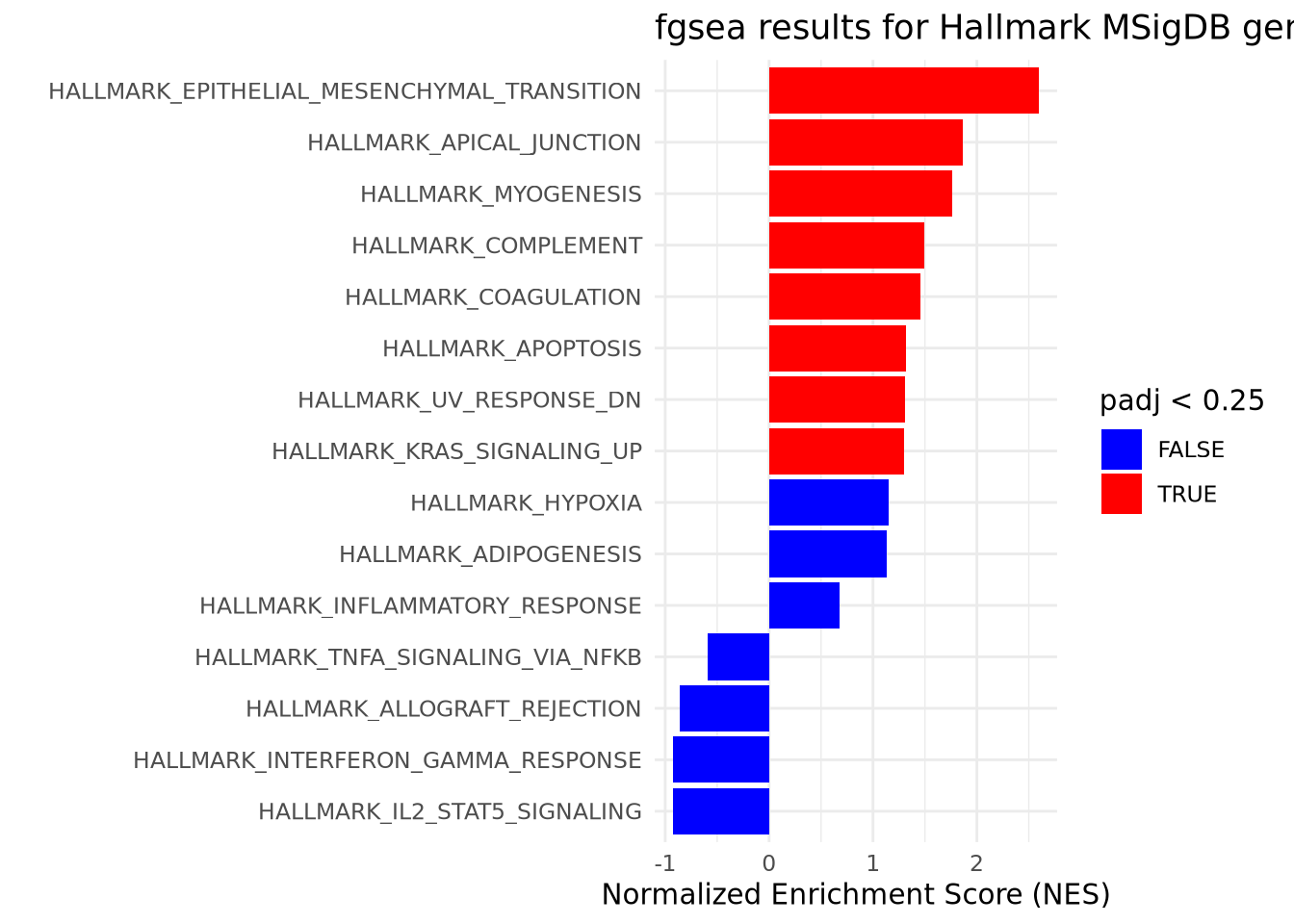
(#fig:top level results plot)GSEA results suggest an enrichment of cancer-related pathways amongst upregulated genes. GSEA was performed using a list of genes generated through RNAseq and ranked by descending fold change. GSEA was run using default parameters with minSize = 15 and maxSize = 500. Gene sets with a Benjamini-Hochberg adjusted p-value < .25 are considered significant.
Given the artificial nature of our data and our choice of a small gene set collection, we have very few results and are able to display all of them intelligibly on one plot. In real experiments, there may be several hundred significant gene sets of interest. In cases like this, you may need to restrict the number of gene sets by taking the top ten ranked by NES (both positive and negative) and plotting those in a figure like the one above. This is only a suggestion and there are many ways to choose ‘interesting’ gene sets to plot together depending upon the experimental context and future questions of interest.
If we wished to investigate a single gene set from this list of results, we
could create an enrichment plot displaying the Enrichment Score as it’s
calculated through the ranked list. For convenience, we have wrapped the
pre-built function, plotEnrichment from fgsea, in a user-defined function that
allows us to specify a specific pathway. The plotEnrichment function expects
at minimum the list of genes contained within the pathway to plot and the input
ranked list of gene-level statistics. We have displayed the enrichment plot for
one of the significantly enriched gene sets below:
make_gsea_plot <- function(pathway_name, rnks) {
plotEnrichment(hallmark_pathways_fgsea[[pathway_name]], rnks) +
    labs(title=pathway_name)
}
make_gsea_plot('HALLMARK_EPITHELIAL_MESENCHYMAL_TRANSITION', rnk_list)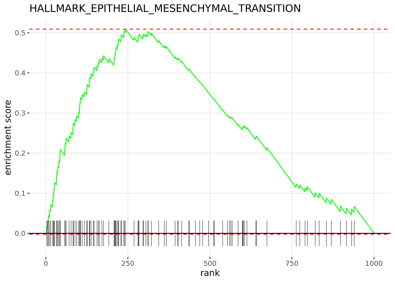
(#fig:enrichment plot)The Hallmarks EPITHELIAL_MESENCHYMAL_TRANSITION Pathway is significantly enriched amongst the upregulated genes. There are 56 genes in the leading edge subset including GAS1, POSTN, and LOX. The Normalized Enrichment Score calculated for this gene set was 2.59 and it has an adjusted p-value of 7.28e-10
As mentioned in the prior section, it is often useful for further investigation
to inspect the leading edge subset of genes contained within ‘interesting’ gene
sets. fgsea stores these genes in the form of a list associated with each
pathway in the returned table. We could convert and save these values in a named
list for convenience. This can be accomplished by making use of the deframe()
function. Below we have saved all of the genes contained within the leading edge
subset of significant gene sets, and displayed those belonging to the
HALLMARK_EPITHELIAL_MESENCHYMAL_TRANSITION gene set as determined in this
experiment:
gather_leadingedge <- function(results, threshold) {

  genes <- results %>%
  filter(padj < threshold) %>%
  dplyr::select(pathway, leadingEdge) %>%
  deframe()
  return(genes)
}

leading_edge_genes <- gather_leadingedge(fgsea_results, .25)
leading_edge_genes$HALLMARK_EPITHELIAL_MESENCHYMAL_TRANSITION
## [1] "GAS1" "MGP" "SPOCK1" "EFEMP2" "FERMT2" "FBN1" "TAGLN" "FSTL1"
## [9] "TIMP3" "VIM" "VCAN" "THBS2" "ACTA2" "DCN" "BGN" "NNMT"
## [17] "CALD1" "NTM" "FBLN1" "SPARC" "COL5A2" "MYL9" "SLIT2" "DPYSL3"
## [25] "VEGFC" "COL3A1" "LGALS1" "THY1" "PCOLCE" "ADAM12" "SFRP4" "WIPF1"
## [33] "COL6A3" "CTHRC1" "TIMP1" "TPM2" "FN1" "COL5A1" "PMP22" "MMP2"
## [41] "HTRA1" "COL1A2" "POSTN" "PDGFRB" "EMP3" "MXRA5" "FLNA" "PRRX1"
## [49] "FAP" "LOX" "BASP1" "GREM1" "CCN2" "CDH11" "LUM" "LAMC1"This named list contains all of the leading edge genes for gene sets meeting a
certain padj threshold. We could import these as a GSEABase GeneSetCollection
object for further analyses in R or write them to a file to pass on to
collaborators.
These examples are just some of the ways you can utilize and explore the GSEA
results returned by fgsea. There are also other methods such as the one found in
the built-in function, fgsea::plotGseaTable, that provide other ways to
visualize these results for groups of different gene sets. You can also perform
any number of different filtering and sorting options on the table of results
depending upon your interests.