Project 2: RNAseq
The projects are broken up into week-by-week sections. However, these sections are guidelines and not a strict timeline. Your report and project will be due only at the day specified on the schedule. These sections are designed to fit a manageable number of tasks into each week and give you a rough timeline.
Docker images for your pipeline
FastQC: ghcr.io/bf528/fastqc:latest
multiQC: ghcr.io/bf528/multiqc:latest
VERSE: ghcr.io/bf528/verse:latest
STAR: ghcr.io/bf528/star:latest
Pandas: ghcr.io/bf528/pandas:latest
Week 1: RNAseq
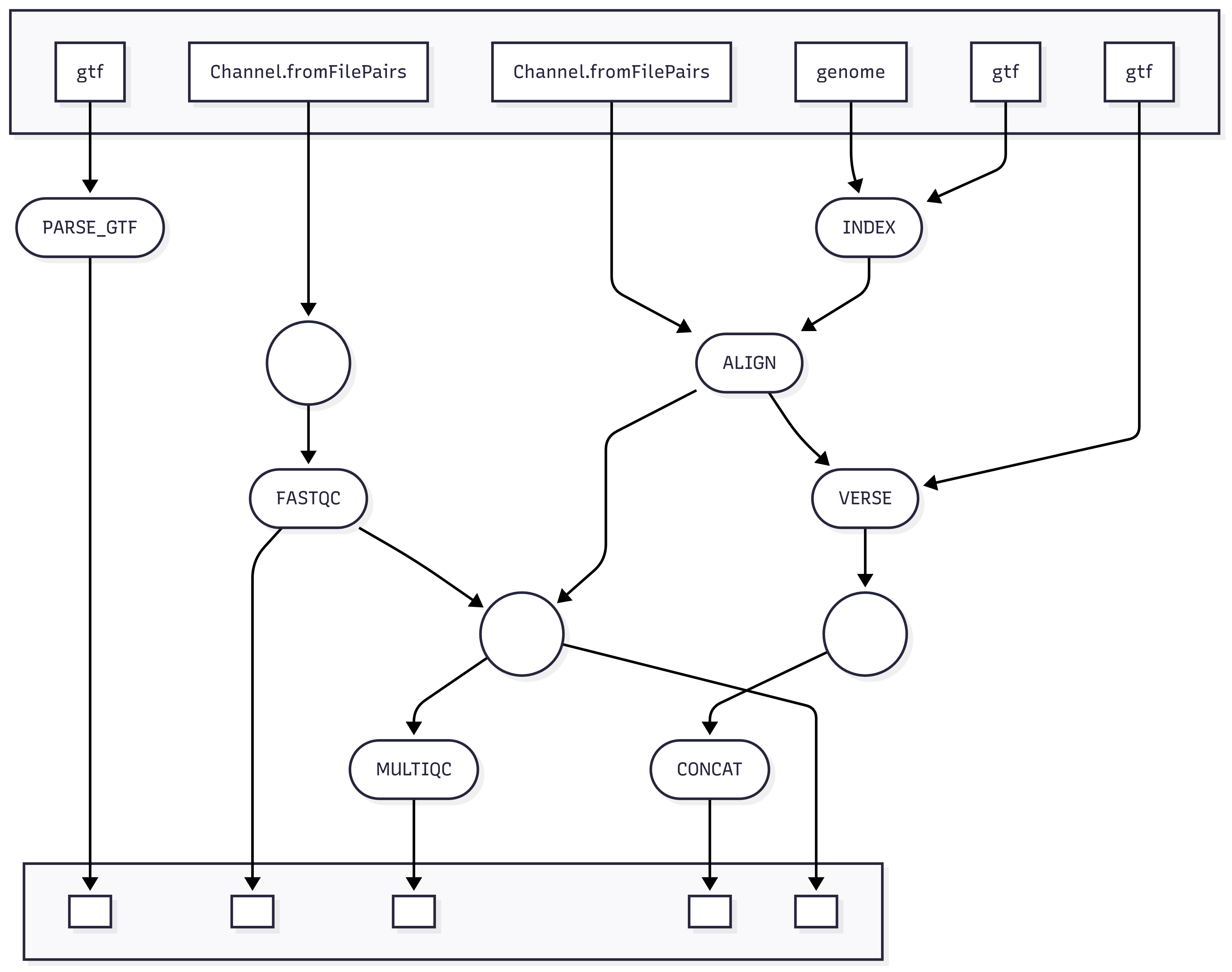
Workflow Visualization
Overview
A basic RNAseq analysis consists of sample quality control, alignment, quantification and differential expression analysis. This week, we will be performing quality control analysis on the sequencing reads, generating a genome index for alignment, and making a mapping of human ensembl IDs to gene names.
Objectives
-
Perform basic quality control by running FASTQC on the sequencing reads
-
Generate a delimited file containing the mapping of human ensembl ids to gene names
-
Use STAR to create a genome index for the human reference genome
Create a working directory for project 1
Accept the github classroom link and clone the assignment to your student directory in /projectnb/bf528/students/your_username/. This link will be posted on the blackboard site for our class.
Necessary paths and files are in your nextflow.config
Please look in your nextflow.config for various variables that I have given you that you will need to use in your pipeline. I have provided you the path to the files as well as the reference genome and matching GTF.
Changes to our environment management strategy and workflow
As we’ve discussed, conda environments are one solution to ensuring that your analyses are run in a reproducible and portable manner. Containers are an alternative technology that have a number of advantages over conda environments. Going forward, we will be incorporating containers specifying our computational environments into our pipeline.
One of the advantages of container technologies is that they usually offer a robust ecosystem of shared containers (images) that are available in public repositories for anyone to reuse. We have developed a set of containers for each piece of software that we will be using in this course.
For all future process scripts that you develop in nextflow, instead of
specifying the conda environment to execute the task with, you will instead
specify container and the image (a container built with a certain specification)
location. For example:
process FASTQC {
  container 'ghcr.io/bf528/fastqc:latest'
  ...

}
For this course, these containers were all pre-built and their specifications kept in this public github repository: https://github.com/BF528/pipeline_containers. Feel free to look into the repo for how the containers were built. We follow a similar pattern where we specify the exact environment we would like created in a YAML file and then generate the environment using micromamba installed in a container. We will get some experience later in the semester with building your own containers from scratch.
In general, the containers will be named following the same pattern:
ghcr.io/bf528/<name-of-tool>:latest or ghcr.io/bf528/fastqc:latest.
New command for running your workflow
You will need to incorporate one more change to make your pipeline use these
containers. If you look in the nextflow.config, you’ll see a profile labeled
singularity, which encodes some singularity options for nextflow to use.
When running your pipeline, you will now use the -profile singularity,local
option, which will have Nextflow execute tasks with the specified container image
listed in the module. The config contains some common options that nextflow will
automatically add to the singularity command when run with the specified profile.
nextflow run main.nf -profile singularity,local
As always, remember to activate your conda environment containing nextflow before running your pipeline.
Generating our input channels for nextflow
This RNAseq pipeline will be driven by two channels that contain the starting
FASTQ files for each of the samples in the experiment. Nextflow has a built-in
function to simplify the generation of channels for samples from paired-end
sequencing experiments. The Channel.fromFilePairs channel function allows you
to detect paired end fastq files for each sample using similar pattern matching
in bash through the use of wildcard expansion (*).
-
In the
nextflow.config, specify a parameter calledreadsthat encodes the path to your fastq files and uses * to flexibly detect the sample name associated with both paired files. Refer to the nextflow documentation here Our files are located at /projectnb/bf528/materials/project_2_rnaseq/subsampled_files/ for the subsampled files. -
In your workflow
main.nf, use theChannel.fromFilePairsfunction and the param you created in step 1 to create a channel calledalign_ch. You’ll notice that this function creates a channel with a structure we’ve seen before: a tuple containing the base name of the file and a list containing the R1 and R2 file associated with that sample.
align_ch

[sample1, [sample1_R1.fastq.gz, sample1_R2.fastq.gz]]
- In your workflow
main.nfcreate another channel using the exact logic from above but add an additional operation to create a channel that has as many elements in the channel as there are actual files (16). You may find information on common nextflow operators that will enable this here
Name this channel fastqc_channel and it should be a list tuples where the
first value is the name of the sample and the second is the path to the
associated file. This will look something like below:
fastqc_channel

[sample1, sample1_R1.fastq.gz]
[sample1, sample1_R2.fastq.gz]
Performing Quality Control
At this point, you should have:
-
Setup a directory for this project by accepting the github classroom link
-
Familiarized yourself with the changes to environment management and how to run nextflow using containers
-
Generate two channels in your
main.nfwith the size and elements specified above
We will begin by performing quality control on the FASTQ files generated from the experiment. fastQC is a bioinformatics software tool that calculates and generates descriptive graphics of the various quality metrics encoded in a FASTQ file. We will use this tool to quickly check the basic quality of the sequencing in this experiment.
- Make a new process for fastqc in the
modules/directory. Be sure to specify the following in your module:
label 'process_low'
container 'ghcr.io/bf528/fastqc:latest'
publishDir <a param containing the path to results/>
- Specify the inputs of the process to match the structure of the
fastqc_channelwe just generated.For this module, please list two named outputs, which will later allow us to use the individual outputs separately:
output:
tuple val(name), path('*.zip'), emit: zip
tuple val(name), path('*.html'), emit: html
This output definition will instruct nextflow that both of these files should exist after FASTQC has run successfully. It will capture the html report and zip file separately and allow you to pass these different values through channels separately (i.e. FASTQC.out.zip would refer specifically to the zip file created by the FASTQC task)
Remember you can use wildcard expansions in the path output to flexibly detect files with certain extensions without specifying their full filename.
- The shell command should be the successful fastqc command you ran earlier. Ensure that the following argument is included in your actual fastQC command:
-t $task.cpus
- Incorporate the FASTQC process into your workflow
main.nfand provide it the proper channel.
Generate a file containing the gene IDs and their corresponding human gene symbols
As we’ve discussed, it’s often more intuitive for us to use gene names rather than their IDs. You are likely familiar with seeing genes referenced by their names in the literature, such as BRCA1 or TP53. However, there are many different identifier systems used to label genes, including ensembl gene ids, which are a common and principled way of labeling and identifying genes. These gene IDS tend to be more stable and consistent across references to the organism and are more standardized. Our genes will originally be in the ensembl gene id format, and we will need to convert them to gene names for downstream analysis.
It is often better to extract this information from the GTF file associated with the exact version of the reference genome we are using. This will ensure that our labels are as internally consistent as possible.
Whenever we need to perform operations using custom code, we are going to use
the conventions established in project 1. We will place this script in the bin/
directory and make it executable. We will then create a nextflow module that will
provide the appropriate command line arguments to the script.
-
Generate a python script that parses the GTF file you were provided and creates a delimited file containing the ensembl human ID and its corresponding gene name. Please copy and modify the
argparsecode used in previous scripts to allow the specification of command line arguments. The script should take the GTF as input and output a single text file containing the requested information. -
Create a nextflow module that calls this script and provides the appropriate command line arguments necessary to run it.
-
You may use the biopython (ghcr.io/bf528/biopython:latest) or the pandas (ghcr.io/bf528/pandas:latest) container to run this task as both of these contain a python installation.
-
Incorporate this module to parse the GTF into your workflow
main.nfand pass it the appropriate GTF input encoded as a param.
Creating your own process labels
As we discussed in class, you can request various ranges of computational resources
for your jobs / processes to use through the qsub command and its accompanying
options.
Please refer to the following page for common combinations of options to request specific amounts of resources from nodes on the SCC.
-
By now you have noticed that some modules have a
labeland you can see in thenextflow.configin the profiles section the exact qsub command and options each label requests. -
Create two new labels named
process_mediumandprocess_high. Forprocess_medium, use the correct options to request 8 cores and <= 32GB ram Forprocess_high, set the options to request 16 cores and <= 128GB ram.
You will need to add a clusterOptions line to the process_high to specify the
additional flags.
Generate a genome index
Most alignment algorithms require an index to be generated to make the alignment process more efficient and expedient. These index files are both specific to the tool and the reference genome used to build them. We will be using the STAR aligner, one of the most commonly used alignment tools for RNAseq.
- Read the beginning of the documentation
for how to generate a STAR index.
- Section 2 describe show to create a genome index and you may use the default commands without changing any options
- Remember that you can run multiple commands in the script block of nextflow by
writing them on new lines. You can use the
mkdircommand to create the output directory for the index files and then reference that same directory in the command.
- Generate a module and process that creates a STAR index for our reference genome. This process will require two inputs, the reference genome and the associated GTF file. Ensure that the following are specified in your module:
label 'process_high'
container 'ghcr.io/bf528/star:latest'
- The outputs of this process will be a directory of multiple files that all comprise the index. You will have to create this directory prior to running the STAR command. Use all of the basic options specified in the manual and leave them at their default values. Be sure to also include the following argument in your STAR command:
--runThreadN $task.cpus
-
Incorporate this process into your workflow and pass it the appropriate inputs from your params encoding the path to the reference genome fasta and GTF file.
-
Make sure you submit this particular job to the cluster with the following command:
nextflow run main.nf -profile singularity,cluster
Week 1 Tasks Summary
-
Clone the github classroom link for this project
-
Use the files contained within your
nextflow.config -
Generate a nextflow channel called
align_chthat has 6 total elements where each element is a tuple containing two elements: the name of the sample, and a list of both of the associated paired end files. -
Generate a nextflow channel called
fastqc_channelthat has 12 total elements where each element is a tuple containing two elements: the name of the sample, and one of the FASTQ files. -
Generate a module that successfully runs FASTQC using the
fastqc_channel -
Develop an external script that parses the GTF and writes a delimited file where one column represents the ensembl human IDs and the value in the other column is the associated human gene symbol.
-
Generate a module that successfully creates a STAR index using the params containing the path to your reference genome assembly and GTF
Week 2: RNAseq
Overview
Now that we have performed basic quality control on the FASTQ files, we are going to map them to the human reference genome to generate alignments for each of our sequencing reads. After alignment, we will aggregate the outputs from FASTQC and STAR into a single report summarizing some of the important quality control metrics describing our sequencing reads and the alignments. We will then quantify the alignments in our BAM file to the gene-level using VERSE.
Objectives
-
Align your sequencing reads to the human reference genome using STAR
-
Use MultiQC to generate a single report containing the quality metrics for the sequencing reads and alignments
-
Generate gene-level counts using VERSE for each of the samples
-
Concatenate gene-level counts from each sample into a single counts matrix
Aligning reads to the genome
Last week you generated a STAR index to enable alignment of reads to the human reference genome. This week, you will use this index to align the sequencing reads to the genome.
Remember that paired end reads are almost always used in conjunction with each other (R1 and R2) and that they collectively represent the reads from a single fragment and sample. When we align both of these paired end reads to the genome, we will generate a single set of all valid alignments for the sample.
By default, many alignment programs will output these alignments in SAM format. As discussed in lecture, the BAM format is a compressed version of SAM files that contains the same information. Oftentimes, we will simply choose to generate BAM files in place of SAM files in order to preserve disk space.
- Look at the documentation for STAR and focus on section 3 (pg. 7) for how to use STAR to run a basic mapping job. Construct a working nextflow module that performs basic alignment using STAR.
Your STAR command should include only the following options and all others may be left at their default value:
--runThreadN, --genomeDir, --readFilesIn, --readFilesCommand,
--outFileNamePrefix, --outSAMtype
- At the end of your STAR command, please add the following code:
2> ${name}.Log.final.out
or
STAR --runThreadN <options> --genomeDir <directory> --readFilesIn <reads> --readFilesCommand zcat --outFileNamePrefix <name>. --outSAMtype <option> 2> ${name}.Log.final.out
The 2> redirects the standard error to the log file and this is what will enable
us to collect the alignment statistics from the log file. The ${name} may differ
based on how you have named your input tuples, but you should name the log file
with the same name as the sample identifier.
- Remember that by default, nextflow stores all of the outputs for a specific task in the staged directory in which it ran. Often, we will want to inspect the output files or log files from various processes.
Ensure that your STAR module has two separate named outputs using emit. The two
outputs will be the BAM file and another for the log file generated during
alignment named with the extension .Log.final.out.
- Ensure that you use the
process_highfor thelabeland the appropriate containerghcr.io/bf528/star:latest.
The log file from STAR will allow us to collect certain statistics about the alignment rates that are useful for quality control purposes. As a general rule of thumb, if there were no obvious issues with the sequencing preparation or errors in the alignment, we expect a substantial proportion of our reads to align to the reference genome. For well-annotated and studied genomes like human or mouse, we usually see alignment rates >70-80% for successful NGS experiments. Lower alignment rates are often expected for genomes that have not been sequenced to the same quality and depth as the more commonly used references. Make sure to evaluate these alignment rates in an experiment-specific context as there is no set threshold or cutoff that is appropriate for all cases.
Performing post-alignment QC
Typically after performing alignment, it is good to obtain a few post-alignment quality control metrics to quickly check if there appear to be any major problems with the data. At this step, we will typically evaluate the quality of the reads themselves (PHRED scores, contamination, etc.) along with the alignment rate to the reference genome.
As we’ve discussed, in larger experiments, it will quickly become cumbersome or unfeasible to manually inspect the results for all of our samples individually. Additionally, if we only look at one sample at a time, we may miss larger trends or biases across all of our samples. To solve this issue, we will be making use of MultiQC, which is a tool that simply aggregates the relevant logs and outputs from various bioinformatics utilities into a nicely formatted HTML report.
Since you are working with files that have been intentionally filtered to make them smaller, the actual outputs from fastQC and STAR will be misleading. Do not draw any conclusions from these reports generated on the subsetted data; the results will only be meaningful when you’ve switched to running this pipeline on the full dataset.
- Make a new module that will run
MultiQC. You can specify the label as
process_lowand setpublishDirto yourresults/directory. We will take advantage of the staging directory strategy that nextflow uses to run MultiQC.
By default, MultiQC will simply scan a directory and automatically detect any
of the common output files and logs created by the bioinformatics tools it
supports. For your input, you can simply specify path('*') and it creates
an HTML file as an output.
- The tricky part with running MultiQC and Nextflow is that you will need to gather all of the output files from FASTQC and STAR and ensure that multiqc only runs after all of the samples have been processed by both of these tools.
Use a combination of map(), collect(), mix(), flatten() to create a
single channel that contains a list with all of the output files from FASTQC and
STAR logs for every sample and call it multiqc_ch. Remember that you may access
the outputs of a previous process by using the .out() notation (i.e. ALIGN.out
or FASTQC.out.zip).
See below for an example of what the channel should look like:
**In class, we may have used the .html file as the output for FastQC, multiQC
will need the .zip file. You can either change the output or add another specifically
for the .zip file created by FastQC.
multiqc_channel

[sample1_R1_fastqc.zip, sample1_R2_fastqc.zip, sample1.Log.final.out,
sample2_R1_fastqc.zip, sample2_R2_fastqc.zip, sample2.Log.final.out, ...]
-
Add the MultiQC module to your workflow
main.nfand run MultiQC. MultiQC should run a single time and only after every alignment and fastqc process has finished. -
Ensure that your
multiqc_report.htmlis successfully created and contains the QC information from both FASTQC and STAR for all of your samples. You may open the HTML file through SCC ondemand. -
Make sure to include the
-fflag in your multiqc command.
Quantifying alignments to the genome
In RNAseq, we are interested in quantifying gene expression and comparing that expression across conditions. We have so far generated alignments from the reads from all of our samples to their appropriate reference genome. We will use the information contained within the GTF (what each region of the genome represents) to assign these alignments to features and count them.
For differential expression analysis, our feature of interest will be exons as those are the regions of genes that largely comprise the sequences found in mRNA (which is what we are measuring and what was originally sequenced). We will generate a single count for every gene representing the sum of the union of all alignments falling into every exon annotated to that gene. This gene-level count will be used as a proxy for that gene’s expression in a particular sample.
We will be using VERSE, which is a read counting tool that will quantify alignments into counts based on a feature of interest. VERSE also has built-in strategies for assigning counts hierarchically in the case of overlapping features.
-
Generate a module that runs VERSE on each of your BAM files. You may leave all options at their default parameters. Be sure to include the
-Sflag in your final command. -
The main output of VERSE is the “*.exon.txt” file. Make sure you name each of the VERSE files with the same name as the sample identifier. This file contains two columns, one for the gene name and one for the count. This represents the counts for every gene in the reference genome for this particular sample.
-
Run the VERSE module in your workflow
main.nfand quantify the alignments in each of the BAM files
Concatenating count outputs into a single matrix
After VERSE has run successfully, you will have generated a single set of counts for each of your samples. To perform differential expression analysis, we will need to combine count outputs from each sample into a single file where the rows are the genes and the columns are the sample counts.
- Write a python script that will concatenate all of the verse output files and
write a single counts matrix containing all of your samples. As with any
external script, make it executable with a proper shebang line and use argparse
to allow the incorporation of command line arguments. I suggest you use
pandasfor this task and you can use the pandas containerghcr.io/bf528/pandas:latest.- Look at the structure of the .exon.txt files, and the final counts matrix / CSV should have the same number of rows as the number of genes in the reference genome and the same number of columns as the number of samples.
- Generate a module that runs this script and create a channel in your workflow
main.nfthat consists of all of the VERSE outputs. Incorporate this script into your workflow and Ensure that this module / script only executes after all of the VERSE tasks have finished.
Week 2 Detailed Task Summary
- Generate a module that runs STAR to align reads to a reference genome
- Ensure that you output the alignments in BAM format
- Use all default parameters
- Specify the log file with extension (.Log.final.out) as a nextflow output
-
Make a module that runs MultiQC using a channel that contains all of the FASTQC outputs and all of the STAR output log files
-
Create a module that runs VERSE on all of your output BAM files to generate gene-level counts for all of your samples
- Write a python script that uses
pandasto concatenate all of the VERSE outputs into a single counts matrix. Generate an accompanying nextflow module that runs this python script
Week 3: RNAseq
Overview
By now, your pipeline should execute all of the necessary steps to perform sample quality control, alignment, and quantification. This week, we will focus on re-running the pipeline with the full data files and beginning a basic differential expression analysis.
Objectives
-
Re-run your working pipeline on the full data files
-
Evaluate the QC metrics for the original samples
-
Choose a filtering strategy for your raw counts matrix
-
Perform basic differential expression on your data using DESeq2
-
Generate a sample-to-sample distance plot and PCA plot for your experiment
Switching to the full data
Once you’ve confirmed that your pipeline works end-to-end on the subsampled files, we are going to properly apply our workflow to the original samples. This will require only a few alterations in order to do.
- Edit your
nextflow.configand change the path found in yourparams.readsto reflect the location of your full files (/projectnb/bf528/materials/project-2-rnaseq/full_files/)
- It is very important you ensure your pipeline runs to completion before running it on the full data. When you do run it on the full data, please only run it once!
Make sure to now always submit jobs to the cluster:
nextflow run main.nf -profile singularity,cluster
You may also need to unset the resume = true option in your config, or manually
set resume = false when you attempt to rerun your workflow on the full data.
You may examine the progress and status of your jobs by using the qstat utility
as discussed in lecture and lab.
Evaluate the QC metrics for the full data
After your pipeline has finished, inspect the MultiQC report generated from the full samples.
- In your provided notebook, comment on the general quality of the sequencing reads. Write a paragraph in the style of a publication reporting what you find and any metrics that might be concerning.
Analysis Tasks - Rmarkdown Notebook
You will typically be performing analyses in either a jupyter notebook or Rmarkdown. With the SCC, we will not be able to easily encapsulate R in an isolated environment.
Instead, simply load the R module (on the launch page for VSCode in on-demand)
as you boot your VSCode extension and work in a Rmarkdown notebook. You may install packages
as needed and ensure that you record the versions used with the sessionInfo()
function.
I highly recommend you use Rmarkdown for this project. It will make it much easier for you to generate your report as nearly all of the analysis tasks will be done in R.
Filtering the counts matrix
We will typically filter our counts matrices to remove genes that we believe will be uninformative for the DE analysis. It is important to remember that filtering is subjective and meant to reduce computational time, or remove uninformative rows.
- Choose a filtering strategy and apply it to your counts matrix. In the provided notebook, report the strategy you used and create a plot or a table that demonstrates the effects of your filtering on the counts for all of your samples. Ensure you mention how many genes are present before and after your filtering threshold.
Performing differential expression analysis using the filtered counts
Refer to the DESeq2 vignette on how to perform a basic differential expression analysis. For this dataset, you will simply be testing for differences between the condition (control vs. experimental). Choose an appropriate padj threshold to generate a list of statistically significant differentially expressed genes from your analysis.
You may refer to the official DESeq2 vignette or the BF591 instructions for how to run a basic differential expression analysis.
Perform a basic differential expression analysis and produce the following as well formatted figures:
- A table containing the DESeq2 results for the top ten significant genes
ranked by padj. Your results should have the corresponding gene names for
each gene symbol. You should not need to use bioMart or any other utility,
you have already created a file from when you parsed the GTF that contains
the gene names for each gene symbol.
- Note that this is not your list of differentially expressed genes. This is just a quick figure that displays some of the most differentially expressed genes
-
Choose an appropriate padj threshold and report the number of significant genes remaining that satisfy this threshold. Make sure you filter your list to only contain these genes. This will be the list of genes you should use as input for the DAVID or ENRICHR analysis
- The results from a DAVID or ENRICHR analysis on the significant genes at your chosen padj threshold. Comment in a notebook what results you find most interesting from this analysis.
RNAseq Quality Control Plots
It is common to produce both a PCA plot as well as a sample-to-sample distance matrix from our counts to assist us in our confidence in whether the differences we see in the differential expression analysis can likely be contributed to our biological condition of interest. All of these plots have convenient wrapper functions already implemented in DESeq2 (see the vignette).
-
Choose an appropriate normalization strategy (rlog or vst) and generate a normalized counts matrix for the experiment. Refer to the DESeq2 vignette here for specific directions on how to do this,
-
Perform PCA on this normalized counts matrix and overlay the sample information in a biplot of PC1 vs. PC2
-
Create a heatmap or graphic of the sample-to-sample distances for the experiment
-
In a notebook, comment in no less than two paragraphs about your interpretations of these plots and what they indicate about the samples, and the experiment.
FGSEA Analysis
Perform a GSEA analysis on your RNAseq results. You are free to use any method available though we recommend fgsea. Please refer to the following resources:
To do this, you will need to do a few steps:
-
Choose an appropriate ranking metric (I suggest log2FoldChange) and create a ranked list of your genes and log2FoldChange in descending order. N.B. For GSEA specifically, you should not filter by significance and your list should be every gene discovered in the experiment.
-
Go to the the C2 canonical pathways MSIGDB dataset and download it to your local computer and upload it to your working directory on the cluster
-
Use either GSEABase or the fgsea function to read in the gene set file (.gmt)
-
Run fgsea using default parameters
-
Using a statistical threshold of your choice, generate a figure or plot that displays the top most significant results from the FGSEA results.
-
In your notebook, briefly remark on your results and what seems interesting to you about the biology.
Week 4: RNAseq
Overview
For the final week, use this time to finish up any tasks you weren’t able to complete. There are no nextflow tasks this week, but you will be asked to create some figures from the original paper using your own findings. Do all of these tasks in the notebook you created from week 3.
Objectives
-
Read the original publication with a specific focus on their RNAseq experiment
-
Reproduce figures 3C and 3F with your own findings and compare them in your discussion
-
Write a short methods section for your pipeline and compare with the methods published in the original paper
Read the original paper
The original publication was given to you in a post on blackboard. Please read the paper and focus specifically on their analysis and discussion of their RNAseq experiment.
Replicate figure 3C and 3F
Focus on figure 3C and specifically their discussion of their RNAseq results.
-
Create a volcano plot similar to the one seen in figure 3c. Use your DAVID or GSEA results and create a plot with the same information as 3F using your findings.
-
Read their discussion of their results and specifically address the following in your provided notebook:
-
Compare how many significant genes are up- and down-regulated in their findings and yours (using their significance threshold). Ensure you list how many you find vs. how many they report.
-
Compare their enrichment results with your DAVID and GSEA analysis. Comment on any differences you observe and why there are discrepancies.
Week 4 Detailed Tasks Summary
-
Read the original publication and focus specifically on the RNAseq experiment
-
Recreate figures 3C and 3F with your own results and ensure you address the listed questions in your notebook
-
Write a methods section in the style we’ve discussed for your workflow
-
Ensure you read the Project 2 Report Guidelines for a full description of what is expected of you.
REMINDER TO CLEAN UP YOUR WORKING DIRECTORY
When you have successfully run your project 2 pipeline, please ensure that you fully delete your work/ directory and any large files that you may have published to your results/ directory.
You may use the following command:
rm -rf work/
These samples are very large and we have limited disk space. I will be checking your working directories to ensure you do this.