R in Biology
R in Biology
- R rose in popularity when microarray technology came into widespread use
- A community of biological researchers and data analysts created a collection of software packages called Bioconductor
- R packages form a bridge between:
- biologists without a computational background and
- statisticians and bioinformaticians, who invent new methods and implement the as R packages that are easily accessible by all
Biological Data Overview
Types of Biological Data
- There are five types of data used in biological data analysis:
- raw/primary data
- processed data
- analysis results
- metadata
- annotation data
Raw/primary data
- The primary observations made by instruments/experiments
- Examples:
- high-throughput sequencing data
- mass/charge ratio data from mass spectrometry
- 16S rRNA sequencing data from metagenomic studies
- SNPs from genotyping assays,
- Often very large and not efficiently processed using R
- Specialized tools built outside of R are used to first process the primary data into a form that is amenable to analysis
- The most common primary biological data types include Microarrays, High Throughput Sequencing data, and mass spectrometry data
Processed data
- The result of any analysis or transformation of primary data into an intermediate, more interpretable form
- For example, in RNASeq:
- short reads aligned against a genome
- counted against annotated genes
- counts form counts matrix of genes x samples
- Processed data does not need to be stored long term if the raw data and code to produce it is available
Analysis results
- Analysis results aren’t data per se but are the results of analysis of primary data or processed data
- Usually what we use to form interpretations of our datasets
- Therefore we must manipulate them in much the same way as any other dataset
Metadata
- Experiments usually study multiple samples
- Each sample typically has information associated with it
- “Data that is about data” is called metadata
- E.g. the information about human subjects included in a study including age at death, whether the person had a disease, the measurements of tissue quality, etc. is the metadata
- The primary and processed data and metadata are usually stored in different files, where the metadata (or sample information or sample data, etc) will have one column indicating the unique identifier (ID) of each sample.
- The processed data will typically have columns named for each of the sample IDs
Annotation data
- Includes previously determined information about biological entities, e.g. genes
- Annotation data is publicly available information about the features we measure in our experiments
- Examples:
- genomic coordinates where genes exist
- any known functions of those genes
- the domains found in proteins and their relative sequence
- gene identifier cross references across different gene naming systems
- single nucleotide polymorphism genomic locations and associations with traits or diseases
Information flow in biological data analysis

CSV Files
CSV Files
csv- character separated value file- Most common, convenient, and flexible data file format in biology and bioinformatics
- Plain text files that contain rectangular data
- Each line of these files has some number of data values separated by a consistent character
- most commonly the comma which are called comma-separated value, or “CSV”, files
- Filenames typically end with the extension
.csv - Other characters, especially the
character, may be used to create valid files in this format
Example CSV file
id,somevalue,category,genes 1,2.123,A,APOE 4,5.123,B,"HOXA1,HOXB1" 7,8.123,,SNCA
Properties and principles of CSV files
- The first line often but not always contains the column names of each column
- Each value is delimited by the same character, in this case
, - Values can be any value, including numbers and characters
- When a value contains the delimiting character (e.g. HOXA1,HOXB1 contains a
,), the value is wrapped in double quotes - Values can be missing, indicated by sequential delimiters (i.e.
,,or one,at the end of the line, if the last column value is missing) - There is no delimiter at the end of the lines
- To be well-formatted every line must have the same number of delimited values
Forms of Biological Data
Common Biological Data Matrices
- processed data typically what we worked with in R
- Common features:
- First row is column headers/sample names
- First column is some identifier (gene symbol, genomic locus, etc)
- Each row is a variable with sample values as columns
Biological Data Matrix Example
intensities <- readr::read_csv("example_intensity_data.csv")
intensities
# A tibble: 54,675 x 36
probe GSM972389 GSM972390 GSM972396 GSM972401 GSM972409
<chr> <dbl> <dbl> <dbl> <dbl> <dbl>
1 1007_s_at 9.54 10.2 9.72 9.68 9.35
2 1053_at 7.62 7.92 7.17 7.24 8.20
3 117_at 5.50 5.56 5.06 7.44 5.19
4 121_at 7.27 7.96 7.42 7.34 7.49
5 1255_g_at 2.79 3.10 2.78 2.91 3.02
# ... with 54,665 more rows, and 26 more variables: GSM972433 <dbl>
# GSM972487 <dbl>, GSM972488 <dbl>, GSM972489 <dbl>,
# GSM972510 <dbl>, GSM972512 <dbl>, GSM972521 <dbl>
Biological data is NOT Tidy!
“tidy” data has the following properties:
- Each variable must have its own column
- Each observation must have its own row
- Each value must have its own cell
Data from high throughput biological experiments have many more variables than observations!
Biological data matrices are usually transposed
- variables as rows
- observations (i.e. samples) as columns
Biological data is NOT Tidy!
# A tibble: 54,675 x 36 probe GSM972389 GSM972390 GSM972396 GSM972401 GSM972409 <chr> <dbl> <dbl> <dbl> <dbl> <dbl> 1 1007_s_at 9.54 10.2 9.72 9.68 9.35 2 1053_at 7.62 7.92 7.17 7.24 8.20
Tidyverse works on tidy data
Base R and tidyverse are optimized to perform computations on columns not rows
Can perform operations on rows rather than columns, but code may perform poorly
A couple options:
Pivot into long format.
Compute row-wise statistics using
apply().intensity_variance <- apply(intensities, 2, var) intensities$variance <- intensity_variance
Bioconductor
Bioconductor
- Bioconductor is an organized collection of strictly biological analysis methods packages
- Hosted and maintained outside of CRAN
- Maintainers enforce rigorous coding quality, testing, and documentation standards
- Bioconductor is divided into roughly two sets of packages:
- core maintainer packages
- user contributed packages
Bioconductor: Core maintainer packages
- Core maintainer packages define a set of common objects and classes e.g.:
- ExpressionSet class in the Biobase package)
- All Bioconductor packages must use these common objects and classes
- Ensures consistency among all Bioconductor packages
Installing Bioconductor
Bioconductor is itself a package called BiocManager
BiocManagermust be installed prior to installing other Bioconductor packagesTo [install bioconductor] (note
install.packages()):if (!require("BiocManager", quietly = TRUE)) install.packages("BiocManager") BiocManager::install(version = "3.16")
Installing Bioconductor packages
# installs the affy bioconductor package for microarray analysis
BiocManager::install("affy")
Bioconductor package pages

Bioconductor documentation
In addition, Biconductor provides three types of documentation:
- Workflow tutorials on how to perform specific analysis use cases
- Package vignettes for every package, provides worked example of how to use the package
- Detailed, consistently formatted reference documentation that gives precise information on functionality and use of each package
Base Bioconductor Packages & Classes
- Base Bioconductor packages define convenient data structures for storing and analyzing biological data
- The
SummarizedExperimentclass stores data and metadata for an experiment
SummarizedExperiment Illustration
SummarizedExperiment Details
SummarizedExperimentclass is used ubiquitously throughout the Bioconductor package ecosystemSummarizedExperimentstores:- Processed data (
assays) - Metadata (
colDataandexptData) - Annotation data (
rowData)
- Processed data (
Microarrays
Microarrays

- Microarrays: devices that measure relative abundance of DNA molecules
- Measure 1000s of DNA molecules simultaneously
- Molecules are selected a priori and “hard coded” onto the device
Microarray Design

Types of Microarrays
- Microarrays measure DNA
- Usually one microarray is generated for an individual sample
- Sample preparation method depends on target molecules
- DNA: e.g. genetic variants, the DNA itself is biochemically extracted
- RNA abundance: RNA extracted then reverse transcribed to complementary DNA (cDNA)
Microarray Terminology
- probe - short (~25nt) cDNA molecule complementary to portion of target transcript
- probe set - a set of probes that all target the same gene
- flowcell - the glass slide portion of device that has probes deposited on it
Microarray Data Generation Process

High Throughput Sequencing
High Throughput Sequencing
- High throughput sequencing (HTS) technologies measure and digitize the nucleotide sequences of thousands to billions of DNA molecules simultaneously
- HTS instruments can determine sequence of any DNA molecule in a sample
- HTS datasets sometimes called unbiased assays
- Most popular HTS technology today is provided by Illumina biotechnology company
Sequencing by synthesis
- Illumina sequencing uses biotechnological technique called sequencing by synthesis
- Sequencing instruments are called sequencers
- The process, briefly:
- \(10^7\) to \(10^9\) short (~300 nucleotide long) DNA molecules ligated to glass slide
- Denatured to become single stranded,
- Complementary strand by incorporating fluorescently tagged nucleotides
- Tagged nucleotides excited by a laser and photograph taken of slide
- Images are processed to reconstruct DNA sequences from fluorescence events
HTS Measures DNA
Any DNA molecules may be subjected to sequencing via this method
Many different types of experiments are possible:
- Whole genome sequencing (WGS)
- RNA Sequencing (RNASeq)
- Whole genome bisulfite sequencing (WGBS)
- Chromatin immunoprecipitation followed by sequencing (ChIPSeq)
Each of these experiments create the same type of data
Each must be interpreted appropriately based on experiment
Raw HTS Data
- Raw HTS data are the digitized DNA sequences for the billions of molecules captured by the flow cell
- Each digitized nucleotide sequence is called a read
- Data stored in a standardized format called the FASTQ file format
FASTQ Format
- Data for a single read in FASTQ format:
@SEQ_ID GATTTGGGGTTCAAAGCAGTATCGATCAAATAGTAAATCCATTTGTTCAACTCACAGTTT + !''*((((***+))%%%++)(%%%%).1***-+*''))**55CCF>>>>>>CCCCCCC65
@- header, unique read name per flowcellGAT...- the nucleotide sequence+- second header, usually blank!''...- the phred quality scores for each base in the read
HTS Sequence Analysis
- Raw sequencing reads must be processed with bioinformatic algorithms
- Two broad classes of sequence analysis:
- de novo assembly to recover complete length of original molecules
- sequence alignment against a set of reference sequences, e.g. genome
- Most data we analyze in R comes from aligned reads that have been produced by other software
Sequence Alignment
- Reads aligned to a reference sequence form a distribution of read counts across all locations in the reference sequence
- Any given reference sequence location, or locus, has zero or more reads that align to it
- The number of reads aligning to a given locus is called the read count
- The read count is proportional to the copy number of molecules in the sample that correspond to that locus
- Read counts from all genes in a reference genome form count data

Count Data
The read counts that align to each locus of a genome form a distribution
Count data have two important properties:
- Count data are integers
- Counts are non-negative
count data are not normally distributed
Analyzing Count Data
Techniques that assume data are normally distributed (like linear regression) are not appropriate for count data
Must account for this in one of two ways:
- Use statistical methods that model counts data - generalized linear models that model data using Poisson and Negative Binomial distributions
- Transform the data to have be normally distributed - certain statistical transformations, such as regularized log or rank transformations can make counts data more closely follow a normal distribution
Gene Identifiers
Gene Identifier Systems
- First gene sequence determined in 1965 - an alanine tRNA in yeast
- Genes are distinct entities - how do we name them?
- In 1979, formal guidelines for human gene nomenclature proposal gave researchers a common vocabulary for genes
- In 1989, Human Genome Organisation (HUGO), become HUGO Gene Nomenclature Committee (HGNC)
- HGNC remains the official body providing guidelines and gene naming authority
- HGNC gene names called gene symbols
HGNC Gene Name Guidelines
- Each gene is assigned a unique symbol, HGNC ID and descriptive name.
- Symbols contain only uppercase Latin letters and Arabic numerals.
- Symbols should not be the same as commonly used abbreviations
- Nomenclature should not contain reference to any species or “G” for gene.
- Nomenclature should not be offensive or pejorative.
Gene Symbols
- Gene symbols are the most human-readable system for naming genes
- e.g. BRCA1, APOE, and ACE2
- Symbols are convenient for humans when reading, identifying, communicating about genes
- However, symbols may be ambiguous, and some genes have many synonymous symbols
- Other gene identifier systems evolved in parallel to address this ambiguity
Gene symbol ambiguity: APOE

Human Gene Identifier Systems: Ensembl
- Ensembl Project genome browser and genome annotation database
- Assigns automatic, systematic ID called Ensembl Gene ID during genome annotation
- Ensembl Gene ID follows convention
ENSGNNNNNNNNNNN, whereNare numbers- e.g. APOE is
ENSG00000130203
- e.g. APOE is
- Gene annotation is
- Supports versions of genes, e.g.
ENSG00000130203.10where.10indicates this is the 10th updated version of this gene - Previous versions maintained
Ensembl Gene IDs for Non-humans
- Ensembl Gene IDs have organism-specific conventions:
| Gene ID Prefix | Organism | Symbol | Example |
|---|---|---|---|
ENSG |
Homo sapiens | HOXA1 | ENSG00000105991 |
ENSMUSG |
Mus musculus (mouse) | Hoxa1 | ENSMUSG00000029844 |
ENSDARG |
Danio rario (zebrafish) | hoxa1a | ENSDARG00000104307 |
ENSFCAG |
Felis catus (cat) | HOXA1 | ENSFCAG00000007937 |
ENSMMUG |
Macaca mulata (macaque) | HOXA1 | ENSMMUG00000012807 |
Other Identifier Systems
- Ensembl is not the only gene identifier system besides gene symbol
- Entrez Gene IDs (UCSC Gene IDs) used by the NCBI Gene database are unique integers for each gene in each organism
- APOE in humans is
384, in mouse11816
- APOE in humans is
- Online Mendelian Inheritance in Man (OMIM) database has identifiers that look like
OMIM:NNNNN, where each OMIM ID refers to a unique gene or human phenotype- APOE is
OMIM:107741
- APOE is
- UniProtKB/Swiss-Prot are protein sequence databases
- APOE is
P02649
- APOE is
Mapping Between Identifier Systems
- Often must map between identifier systems
- e.g. We have Ensembl Gene ID, but want gene symbols
- Ensembl provides BioMart that provides gene identifier mappings
- Mappings can be downloaded as CSV files
- Ensembl website has helpful documentation on how to use BioMart to download annotation data
Biomart in Bioconductor: biomaRt
- Ensembl also provides the
biomaRtBioconductor package - Allows programmatic access to the same information directly from R
- There is much more information in the Ensembl databases than gene annotation data that can be accessed via BioMart
biomaRt Example
# this assumes biomaRt is already installed through bioconductor library(biomaRt) # the human biomaRt database is named "hsapiens_gene_ensembl" ensembl <- useEnsembl(biomart="ensembl", dataset="hsapiens_gene_ensembl")
biomaRt Example
# listAttributes() returns a data frame, convert to tibble as_tibble(listAttributes(ensembl)) # A tibble: 3,143 x 3 name description page <chr> <chr> <chr> 1 ensembl_gene_id Gene stable ID feature_page 2 ensembl_gene_id_version Gene stable ID version feature_page 3 ensembl_transcript_id Transcript stable ID feature_page 4 ensembl_transcript_id_version Transcript stable ID version feature_page 5 ensembl_peptide_id Protein stable ID feature_page 6 ensembl_peptide_id_version Protein stable ID version feature_page 7 ensembl_exon_id Exon stable ID feature_page 8 description Gene description feature_page 9 chromosome_name Chromosome/scaffold name feature_page 10 start_position Gene start (bp) feature_page # ... with 3,133 more rows
biomaRt Example
namecolumn provides programmatic name associated with the attribute that can be used to retrieve that annotation information using thegetBM()function:
# create a tibble with ensembl gene ID, HGNC gene symbol, and gene description
gene_map <- as_tibble(
getBM(
attributes=c("ensembl_gene_id", "hgnc_symbol", "description"),
mart=ensembl
)
)
biomaRt Example
gene_map # A tibble: 68,012 x 3 ensembl_gene_id hgnc_symbol description <chr> <chr> <chr> 1 ENSG00000210049 MT-TF mitochondrially encoded tRNA-Phe ... 2 ENSG00000211459 MT-RNR1 mitochondrially encoded 12S rRNA ... 3 ENSG00000210077 MT-TV mitochondrially encoded tRNA-Val ... 4 ENSG00000210082 MT-RNR2 mitochondrially encoded 16S rRNA ... 5 ENSG00000209082 MT-TL1 mitochondrially encoded tRNA-Leu ... 6 ENSG00000198888 MT-ND1 mitochondrially encoded NADH:ubiquinone 7 ENSG00000210100 MT-TI mitochondrially encoded tRNA-Ile ... 8 ENSG00000210107 MT-TQ mitochondrially encoded tRNA-Gln ... 9 ENSG00000210112 MT-TM mitochondrially encoded tRNA-Met ... 10 ENSG00000198763 MT-ND2 mitochondrially encoded NADH:ubiquinone # ... with 68,002 more rows
Mapping Homologs
Many organisms share evolutionarily conserved genes (i.e. homologs)
biomaRtlinks identifiers by explicitly connecting different biomaRt databases with thegetLDS()function:human_db <- useEnsembl("ensembl", dataset = "hsapiens_gene_ensembl") mouse_db <- useEnsembl("ensembl", dataset = "mmusculus_gene_ensembl") orth_map <- as_tibble( getLDS(attributes = c("ensembl_gene_id", "hgnc_symbol"), mart = human_db, attributesL = c("ensembl_gene_id", "mgi_symbol"), martL = mouse_db ) )
Mapping Homologs
orth_map # A tibble: 26,390 x 4 Gene.stable.ID HGNC.symbol Gene.stable.ID.1 MGI.symbol <chr> <chr> <chr> <chr> 1 ENSG00000198695 MT-ND6 ENSMUSG00000064368 "mt-Nd6" 2 ENSG00000212907 MT-ND4L ENSMUSG00000065947 "mt-Nd4l" 3 ENSG00000279169 PRAMEF13 ENSMUSG00000094303 "" 4 ENSG00000279169 PRAMEF13 ENSMUSG00000094722 "" 5 ENSG00000279169 PRAMEF13 ENSMUSG00000095666 "" 6 ENSG00000279169 PRAMEF13 ENSMUSG00000094741 "" 7 ENSG00000279169 PRAMEF13 ENSMUSG00000094836 "" 8 ENSG00000279169 PRAMEF13 ENSMUSG00000074720 "" 9 ENSG00000279169 PRAMEF13 ENSMUSG00000096236 "" 10 ENSG00000198763 MT-ND2 ENSMUSG00000064345 "mt-Nd2" # ... with 26,380 more rows
Alternative: AnnotationDbi
- BioMart/biomaRt is not the only ways to map different gene identifiers
- AnnotateDbi provides gene identifier mapping independent of Ensembl
- Also includes identifiers from technology platforms, e.g. probe set IDs from microarrays
- Also allows comprehensive and flexible homolog mapping
Gene Expression
Gene Expression
- Gene expression: the process by which information from a gene is used in the synthesis of functional gene products that affect a phenotype.
- Gene expression studies are often focused on protein coding genes, there are many other functional molecules, e.g. transfer RNAs, lncRNAs, etc, that are produced by this process. The gene expression process has many steps and intermediate products, as depicted in the following figure:
Gene Expression Process
- Specific parts of the genome code for genes
- Gene sequences transcribed into RNA molecules called transcripts
- In lower organisms (e.g. bacteria), RNA molecules passed directly to ribosomes
- In most higher organisms (i.e. eukaryotes):
- Initial transcripts, called pre-messenger RNA (pre-mRNA) transcripts are processed via splicing
- Splicing removes certain parts of pre-mRNA (introns) and concatenates adjacent sequences (exons) together into mature RNA (mRNA)
- mRNA exported from nucleus to be translated at ribosomes
Gene Expression Process

Gene Expression Measurements
- Measurements proportional to abundance (or copy number) of RNA transcripts
- Measurements are always non-negative
- Usually relative to some normalizing quantity
- i.e. a value of zero does not mean gene is not expressed!
- Some methods (e.g. digital droplet PCR) can estimate absolute abundance (i.e. exact number of copies)
Gene Expression Assays
Many ways to measure the abundance of RNA transcripts
- Light absorbance
- Northern blot
- quantitative polymerase chain reaction (qPCR)
- Oligonucleotide and microarrays
- High throughput RNA sequencing (RNASeq)
Gene Expression Data in Bioconductor
Gene Expression Data in Bioconductor
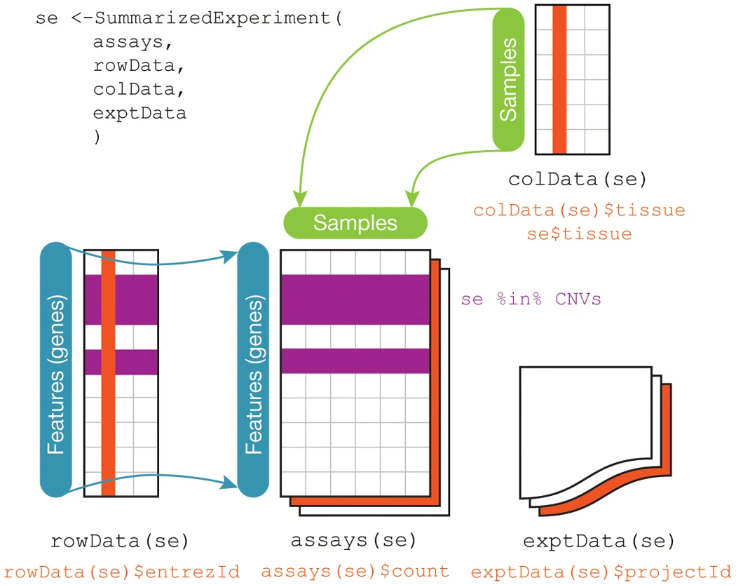
SummarizedExperiment container standard way to load and work with gene expression data in Bioconductor This container requires the following information:
assays- one or more measurement assays (e.g. gene expression) in the form of a feature by sample matrixcolData- metadata associated with the samples (i.e. columns) of the assaysrowData- metadata associated with the features (i.e. rows) of the assaysexptData- additional metadata about the experiment itself, like protocol, project name, etc
SummarizedExperiment Schematic
Creating SummarizedExperiments
- Many Bioconductor packages for specific types of data, e.g. limma create SummarizedExperiment objects for you
- You may also create your own…
Creating SummarizedExperiments
# microarray expression dataset intensities intensities <- readr::read_delim( "example_intensity_data.csv",delim=" " ) # the first column of intensities tibble is the probesetId, # extract to pass as rowData rowData <- intensities["probeset_id"] # remove probeset IDs from tibble and turn into a R dataframe # so that we can assign rownames since tibbles don't support # row names intensities <- as.data.frame( select(intensities, -probeset_id) ) rownames(intensities) <- rowData$probeset_id
SummarizedExperiment cont’d
# these column data are made up, but you would have a
# sample metadata file to use
colData <- tibble(
sample_name=colnames(intensities),
condition=sample(c("case","control"),ncol(intensities),replace=TRUE)
)
se <- SummarizedExperiment(
assays=list(intensities=intensities),
colData=colData,
rowData=rowData
)
SummarizedExperiment cont’d
se ## class: SummarizedExperiment ## dim: 54675 35 ## metadata(0): ## assays(1): intensities ## rownames(54675): 1007_s_at 1053_at ... AFFX-TrpnX-5_at AFFX-TrpnX-M_at ## rowData names(1): probeset_id ## colnames(35): GSM972389 GSM972390 ... GSM972512 GSM972521 ## colData names(2): sample_name condition
Differential Expression Analysis
Differential Expression Analysis
- Goal: identify to what extent gene expression is associated with one or more variables of interest
- Typically analyze whole transcriptome (i.e. 1000s of genes)
- Two required components:
- an expression matrix (e.g. genes x samples)
- a design matrix
The Design Matrix
- A design matrix is a numeric matrix that contains
- the variables we wish to model
- any covariates or confounders we wish to adjust for
- Encoded in a way that statistical procedures understand
- Construct these matrices from a tibble with the
model.matrix()function
Example Metadata
ad_metadata
## # A tibble: 6 × 8 ## ID age_at_death condition tau abeta iba1 gfap braak_stage ## <chr> <dbl> <fct> <dbl> <dbl> <dbl> <dbl> <fct> ## 1 A1 73 AD 96548 176324 157501 78139 4 ## 2 A2 82 AD 95251 0 147637 79348 4 ## 3 A3 82 AD 40287 45365 17655 127131 2 ## 4 C1 80 Control 62684 93739 131595 124075 3 ## 5 C2 77 Control 63598 69838 7189 35597 3 ## 6 C3 72 Control 52951 19444 54673 17221 2
Case vs Control Design
- Model matrix to identify genes that are increased or decreased in people with AD compared with Controls
- The
~ conditionargument is an an R formula
model.matrix(~ condition, data=ad_metadata)
Case vs Control Design
model.matrix(~ condition, data=ad_metadata)
## (Intercept) conditionAD ## 1 1 1 ## 2 1 1 ## 3 1 1 ## 4 1 0 ## 5 1 0 ## 6 1 0 ## attr(,"assign") ## [1] 0 1 ## attr(,"contrasts") ## attr(,"contrasts")$condition ## [1] "contr.treatment"
Formulas in R
The general format of a formula is as follows:
# portions in [] are optional [<outcome variable>] ~ <predictor 1> [+ <predictor 2>]... # examples # model Gene 3 expression as a function of disease status `Gene 3` ~ condition # model the amount of tau pathology as a function of abeta pathology, # adjusting for age at death tau ~ age_at_death + abeta # can create a model without an outcome variable ~ age_at_death + condition
More Complex Designs
- Can include other variables in model to adjust for covariates or test other contrasts
- e.g. adjust out the effect of age by including
age_at_deathas a covariate in the model:
model.matrix(~ age_at_death + condition, data=ad_metadata)
More Complex Designs
model.matrix(~ age_at_death + condition, data=ad_metadata)
## (Intercept) age_at_death conditionAD ## 1 1 73 1 ## 2 1 82 1 ## 3 1 82 1 ## 4 1 80 0 ## 5 1 77 0 ## 6 1 72 0 ## attr(,"assign") ## [1] 0 1 2 ## attr(,"contrasts") ## attr(,"contrasts")$condition ## [1] "contr.treatment"
Microarray Gene Expression Data
Four steps involved in analyzing gene expression microarray data:
- Summarization of probes to probesets
- Normalization
- Quality control
- Analysis
Microarray Data
- Raw probe intensity data stored in CEL data files
affyBioconductor package- Loads CEL files into Bioconductor objects
- Performs key preprocessing operations
- Typically have many CEL files, one per each sample
Reading CEL Files
- Load CEL files with
affy::ReadAffyfunction
# read all CEL files in a single directory affy_batch <- affy::ReadAffy(celfile.path="directory/of/CELfiles") # or individual files in different directories cel_filenames <- c( list.files( path="CELfile_dir1", full.names=TRUE, pattern=".CEL$" ), list.files( path="CELfile_dir2", full.names=TRUE, pattern=".CEL$" ) ) affy_batch <- affy::ReadAffy(filenames=cel_filenames)
Probe summarization and normalization
affypackage provides functions to perform probe summarization and normalization- Robust Multi-array Average (RMA) state of the art method for normalization
affy::rmafunction implements RMA, performs summarization and normalization of multiple arrays simultaneously
Aside: R package data
- Some packages include data with the R functionality
- Load package data into your workspace with
data()function
library(affydata) data(Dilution)
RMA normalization
library(affy) library(affydata) data(Dilution) # normalize the Dilution microarray expression values # note Dilution is an AffyBatch object eset_rma <- affy::rma(Dilution,verbose=FALSE)
ExpressionSet vs SummarizedExperiment
ExpressionSetis a container that contains high throughput assay data- Similar to and superseded by
SummarizedExperiment - Some older packages (notably
affy) returnExpressionSetobjects, notSummarizedExperiments - Similar interface, but some key differences
| Operation | ExpressionSet | SummarizedExperiment |
|---|---|---|
| Get expression values | exprs(eset) |
assays(se) |
| Get column data | phenoData(eset) |
colData(se) |
| Get row data | annotation(eset) |
rowData(se) |
RMA normalization

Differential Expression: Microarrays (limma)
- limma:
linearmodels ofmicroarrays - Designed for analyzing microarray gene expression data
- One of the top most downloaded Bioconductor packages
- Supports arbitrarily complex experimental designs while maintaining strong statistical power
- Can perform reliable inference even with small sample sizes
limma Example Setup
- limma requires:
ExpressionSetorSummarizedExperimentcontainer- a design matrix
ad_se <- SummarizedExperiment( assays=list(intensities=intensities), colData=ad_metadata, rowData=rownames(intensities) ) # design matrix for AD vs control, adjusting for age at death ad_vs_control_model <- model.matrix( ~ age_at_death + condition, data=ad_metadata )
limma Example: fit model
# now run limma # first fit all genes with the model fit <- limma::lmFit( assays(se)$intensities, ad_vs_control_model ) # now better control fit errors with the empirical Bayes method fit <- limma::eBayes(fit)
limma Results
- Look at top results using
limma::topTable()function:
# the coefficient name conditionAD is the column name in the design matrix topTable(fit, coef="conditionAD", adjust="BH", number=5)
## logFC AveExpr t P.Value adj.P.Val B ## 206354_at -2.7507429 5.669691 -5.349105 3.436185e-05 0.9992944 -2.387433 ## 234942_s_at 0.9906708 8.397425 5.206286 4.726372e-05 0.9992944 -2.447456 ## 243618_s_at -0.6879431 7.148455 -4.864695 1.020980e-04 0.9992944 -2.598600 ## 223703_at 0.8693657 6.154392 4.745033 1.340200e-04 0.9992944 -2.654092 ## 244391_at -0.5251423 5.532712 -4.691482 1.514215e-04 0.9992944 -2.679354
RNASeq
RNASeq
- RNA sequencing (RNASeq) digitizes the RNA molecules in a sample
- Short reads (~100-300 nucleotides long) represent RNA fragments from longer transcripts
- RNA molecules are (in principle) sequenced in proportion to their relative copy number in the original sample
- Each sequencing dataset has a total number of reads called library size
- Relative copy number means absence of evidence is not evidence of absence
- i.e. count of zero does not necessarily mean no molecules
RNASeq Gene Expression Data
- When aligned, reads are counted using a reference annotation that defines locations of genes in the genome
- For a single sample, output is a vector of read counts for each gene in the annotation
- Genes with no reads mapping to them will have a count of zero
- All others will have a read count of one or more;
- Complex multicellular organisms have on the order of thousands to tens of thousands of genes
The Counts Matrix
- Read counts from multiple samples of genes using the same annotation are usually concatenated into a counts matrix
- Counts matrix usually has genes as rows and samples as columns (not tidy!)
- Usually in
csvortsv(tab separated) format - These counts are from O’Meara et al 2014
counts <- read_tsv("verse_counts.tsv")
Example Counts Matrix
counts
## # A tibble: 55,416 × 9 ## gene P0_1 P0_2 P4_1 P4_2 P7_1 P7_2 Ad_1 Ad_2 ## <chr> <dbl> <dbl> <dbl> <dbl> <dbl> <dbl> <dbl> <dbl> ## 1 ENSMUSG00000102693.2 0 0 0 0 0 0 0 0 ## 2 ENSMUSG00000064842.3 0 0 0 0 0 0 0 0 ## 3 ENSMUSG00000051951.6 19 24 17 17 17 12 7 5 ## 4 ENSMUSG00000102851.2 0 0 0 0 1 0 0 0 ## 5 ENSMUSG00000103377.2 1 0 0 1 0 1 1 0 ## 6 ENSMUSG00000104017.2 0 3 0 0 0 1 0 0 ## 7 ENSMUSG00000103025.2 0 0 0 0 0 0 0 0 ## 8 ENSMUSG00000089699.2 0 0 0 0 0 0 0 0 ## 9 ENSMUSG00000103201.2 0 0 0 0 0 0 0 1 ## 10 ENSMUSG00000103147.2 0 0 0 0 0 0 0 0 ## # ℹ 55,406 more rows
Analyzing Counts Data
There are typically three steps when analyzing a RNASeq count matrix:
- Filter genes that are unlikely to be differentially expressed.
- Normalize filtered counts to make samples comparable to one another.
- Differential expression analysis of filtered, normalized counts.
Filtering Counts
- Genes not detected in any sample (counts are zero) should not be considered
- Genes with very low counts are not likely to be informative
- Eliminating these genes from consideration reduce multiple hypothesis testing burden later
- General approach: set read count criteria to filter out genes
Filtering Undetected Genes
- Genes not detected in any sample should be filtered
nonzero_genes <- rowSums(counts[-1])!=0 filtered_counts <- counts[nonzero_genes,] slice_head(filtered_counts, n=5)
## # A tibble: 5 × 9 ## gene P0_1 P0_2 P4_1 P4_2 P7_1 P7_2 Ad_1 Ad_2 ## <chr> <dbl> <dbl> <dbl> <dbl> <dbl> <dbl> <dbl> <dbl> ## 1 ENSMUSG00000051951.6 19 24 17 17 17 12 7 5 ## 2 ENSMUSG00000102851.2 0 0 0 0 1 0 0 0 ## 3 ENSMUSG00000103377.2 1 0 0 1 0 1 1 0 ## 4 ENSMUSG00000104017.2 0 3 0 0 0 1 0 0 ## 5 ENSMUSG00000103201.2 0 0 0 0 0 0 0 1
Filtering Very Low Count Genes
- Genes with fewer than 2 reads across all samples filtered
nonzero_genes <- rowSums(counts[-1])>=2 filtered_counts <- counts[nonzero_genes,] slice_head(filtered_counts, n=5)
## # A tibble: 5 × 9 ## gene P0_1 P0_2 P4_1 P4_2 P7_1 P7_2 Ad_1 Ad_2 ## <chr> <dbl> <dbl> <dbl> <dbl> <dbl> <dbl> <dbl> <dbl> ## 1 ENSMUSG00000051951.6 19 24 17 17 17 12 7 5 ## 2 ENSMUSG00000103377.2 1 0 0 1 0 1 1 0 ## 3 ENSMUSG00000104017.2 0 3 0 0 0 1 0 0 ## 4 ENSMUSG00000102331.2 5 8 2 6 6 11 4 3 ## 5 ENSMUSG00000025900.14 4 3 6 7 7 3 36 35
Filtering by Non-zero Sample Counts
- Statistical procedures don’t work with too many zeros
- Small read counts may indicate very lowly abundant but biologically relevant genes
- Can filter genes based on number of non-zero sample counts
- e.g. Filter out genes if they have zero counts in more than half of samples
Filtering by Non-zero Sample Counts

Filtering by Non-zero Sample Counts
- Consider genes present in at least \(n\) samples
- Plots distribution of mean counts within each number of nonzero samples:

Mean-variance Relationship
- In counts data, genes with higher mean count also have higher variance
- Mean-variance dependence means these count data are heteroskedastic

Filtering For Statistics
- Genes with very few counts do not enable reliable statistical inference
- There is no biological meaning to any filtering threshold
- The read counts for a gene depends upon the total number of reads generated
- We cannot use filtering to “remove lowly expressed genes”
- Can only filter out genes that are below the detection threshold afforded by the library size of the dataset
Count Distributions
- The range of gene expression in a cell varies by orders of magnitude
- Consider the distribution of read counts on a log10 scale from one sample
dplyr::select(filtered_counts, Ad_1) %>% filter(Ad_1 > 0) %>% # avoid taking log10(0) mutate(`log10(counts)`=log10(Ad_1)) %>% ggplot(aes(x=`log10(counts+1)`)) + geom_histogram(bins=50) + labs(title='log10(counts) distribution for Adult mouse')
Count Distributions

Count Distributions
- Consider distribution for all the samples as a ridgeline plot

Count Normalization
- Every sample will have a different number of reads (library size)
- The number of reads that maps to any given gene is dependent upon:
- the relative abundance of the molecule in the sample
- the library size of each sample
- The raw read counts are not directly comparable between samples
- Counts in each sample must be normalized so they are comparable
Count Normalization
- Count normalization: the process by which the number of raw counts in each sample is scaled by a factor to make multiple samples comparable
- Many strategies have been proposed to do this
- The simplest is: divide ever count by some factor of the library size
- e.g. compute counts per million reads or CPM normalization
\[ cpm_{s,i} = \frac{c_{s,i}}{l_s} * 10^6 \]
Counts Per Million
\[ cpm_{s,i} = \frac{c_{s,i}}{l_s} * 10^6 \]
- \(c_{s,i} =\) raw count of gene \(i\) in sample \(s\)
- \(l_s =\) library size for sample \(s\)
- In principle, the proportion of read counts for each gene will be comparable between samples
CPM Normalization

Library Size Normalization
- CPM is a library size normalization
- Library size normalizations are sensitive to extreme outlier genes
- e.g. if one gene in one sample has abnormally large counts, this can cause other gene counts to be smaller than they truly are
- These outlier counts are common in RNASeq data!
- Normalization method should be robust to these outliers
DESeq2 Normalization
- DESeq2 bioconductor package introduced a robust normalization method
- Assumes that most genes are not differentially expressed
- Uses the median geometric mean computed across all samples to determine the scale factor for each sample
- Currently the de facto standard normalization method for well characterized genomes
DESeq2 Normalization
library(DESeq2) # DESeq2 requires a counts matrix # column data (sample information), and a formula # the counts matrix *must be raw counts* count_mat <- as.matrix(filtered_counts[-1]) row.names(count_mat) <- filtered_counts$gene dds <- DESeqDataSetFromMatrix( countData=count_mat, colData=tibble(sample_name=colnames(filtered_counts[-1])), design=~1 # no formula needed, ~1 produces a trivial design matrix )
DESeq2 Normalization
# compute normalization factors dds <- estimateSizeFactors(dds) # extract the normalized counts deseq_norm_counts <- as_tibble(counts(dds,normalized=TRUE)) %>% mutate(gene=filtered_counts$gene) %>% relocate(gene) # relocate changes column order
DESeq2 vs CPM

DESeq2 Considerations
The DESeq2 normalization procedure has two important considerations:
- The procedure borrows information across all samples.
- The procedure does not use genes with any zero counts.
The CPM normalization procedure does not borrow information across all samples, and therefore is not subject to these considerations.
Count Transformation
- One way to deal with the non-normality of count data is transform it to follow a normal distribution
- Enables more statistical methods like linear regression to be used
- Count data are roughly log-normal, however low and zero counts can be problematic for traditional
log() - The DESeq2 package provides the
rlog()function that performs a regularized logarithmic transformation that avoids these biases
# the dds is the DESeq2 object from earlier rld <- rlog(dds)
Count Transformation

Differential Expression: RNASeq
- Normalized read counts are suitable for differential expression
- Counts matrix created by concatenating read counts for all genes rows are genes or transcripts and columns are samples
- Read counts not normally distributed, requires statistical approach that either
- Models counts explicitly
- Transform counts to be normally distributed, use common statistical methods
Modeling Count Data
- Poisson distribution: expresses probability that a given number of events occur in a fixed period, e.g. time, space, distance, area, volume
- Can model number of reads aligning to a given genome position/locus
- Whole Genome Sequencing (WGS) data are modeled this way
Poisson Distribution
\[ f(k;\lambda) = \mathtt{Pr}(X=k) = \frac{\lambda^k e^{-\lambda}}{k!} \]
- \(\lambda\) is the average number of events observed in each period
\[ \lambda = \mathtt{E}(X) = \mathtt{Var}(X) \]
- In Poisson, the mean and variance are assumed to be equal
WGS Read Depth

WGS Read Depth Distribution

RNASeq Read Depth

Mean-variance Relationship
- In counts data, genes with higher mean count also have higher variance
Negative Binomial Distribution
- In a set of Bernoulli trials, models the number of failures before a specified number of successes occurs
\[ f(k; r,p) = \mathtt{Pr}(X=k) = \binom{k+r-1}{k} (1-p)^k p^r \]
- \(r\) - number of “successes”, \(p\) - probability of success
- Alternate formulation:
\[ p = \frac{\mu}{\sigma^2}, r = \frac{\mu^2}{\sigma^2 - \mu} \]
DESeq2 Dispersion Estimation
- Index of dispersion \(D\)
\[ D = \frac{\sigma^2}{\mu} \]
DESeq2 Dispersion Estimation

DESeq2/EdgeR
DESeq2
As mentioned briefly above, DESeq2 requires three pieces of information to perform differential expression:
- A raw counts matrix with genes as rows and samples as columns
- A data frame with metadata associated with the columns
- A design formula for the differential expression model
DESeq2 Example
library(DESeq2)
# the counts matrix *must be raw counts*
count_mat <- as.matrix(filtered_counts[-1])
row.names(count_mat) <- filtered_counts$gene
# create a sample matrix from sample names
sample_info <- tibblesample_name=colnames(filtered_counts[-1])) %>%
separate(sample_name,
c("timepoint","replicate"),sep="_",remove=FALSE
) %>%
mutate(
timepoint=factor(timepoint,levels=c("Ad","P0","P4","P7"))
)
design <- formula(~ timepoint)
DESeq2 Example
sample_info
## # A tibble: 8 × 3 ## sample_name timepoint replicate ## <chr> <fct> <chr> ## 1 P0_1 P0 1 ## 2 P0_2 P0 2 ## 3 P4_1 P4 1 ## 4 P4_2 P4 2 ## 5 P7_1 P7 1 ## 6 P7_2 P7 2 ## 7 Ad_1 Ad 1 ## 8 Ad_2 Ad 2
DESeq2 Example
dds <- DESeqDataSetFromMatrix( countData=count_mat, colData=sample_info, design=design ) dds <- DESeq(dds) resultsNames(dds)
## [1] "Intercept" "timepoint_P0_vs_Ad" "timepoint_P4_vs_Ad" ## [4] "timepoint_P7_vs_Ad"
DESeq2 Results
res <- results(dds, name="timepoint_P0_vs_Ad") p0_vs_Ad_de <- as_tibble(res) %>% mutate(gene=rownames(res)) %>% relocate(gene) %>% arrange(pvalue) head(p0_vs_Ad_de, 5)
## # A tibble: 5 × 7 ## gene baseMean log2FoldChange lfcSE stat pvalue padj ## <chr> <dbl> <dbl> <dbl> <dbl> <dbl> <dbl> ## 1 ENSMUSG00000000031.17 19624. 6.75 0.187 36.2 2.79e-286 5.43e-282 ## 2 ENSMUSG00000026418.17 9671. 9.84 0.283 34.7 2.91e-264 2.83e-260 ## 3 ENSMUSG00000051855.16 3462. 5.35 0.155 34.5 4.27e-261 2.76e-257 ## 4 ENSMUSG00000027750.17 9482. 4.05 0.123 33.1 1.23e-239 5.98e-236 ## 5 ENSMUSG00000042828.13 3906. -5.32 0.165 -32.2 3.98e-227 1.55e-223
DESeq2 Results
- baseMean - the mean normalized count of all samples for the gene
- log2FoldChange - the estimated coefficient (i.e. log2FoldChange) for the comparison of interest
- lfcSE - the standard error for the log2FoldChange estimate
- stat - the Wald statistic associated with the log2FoldChange estimate
- pvalue - the nominal p-value of the Wald test (i.e. the signifiance of the association)
- padj - the multiple testing adjusted p-value (i.e. false discovery rate)
Filtering DESeq2 Results
# number of genes significant at FDR < 0.05 filter(p0_vs_Ad_de,padj<0.05)
## # A tibble: 7,467 × 7 ## gene baseMean log2FoldChange lfcSE stat pvalue padj ## <chr> <dbl> <dbl> <dbl> <dbl> <dbl> <dbl> ## 1 ENSMUSG00000000031.17 19624. 6.75 0.187 36.2 2.79e-286 5.43e-282 ## 2 ENSMUSG00000026418.17 9671. 9.84 0.283 34.7 2.91e-264 2.83e-260 ## 3 ENSMUSG00000051855.16 3462. 5.35 0.155 34.5 4.27e-261 2.76e-257 ## 4 ENSMUSG00000027750.17 9482. 4.05 0.123 33.1 1.23e-239 5.98e-236 ## 5 ENSMUSG00000042828.13 3906. -5.32 0.165 -32.2 3.98e-227 1.55e-223 ## 6 ENSMUSG00000046598.16 1154. -6.08 0.197 -30.9 5.77e-210 1.87e-206 ## 7 ENSMUSG00000019817.19 1952. 5.15 0.170 30.3 1.14e-201 3.18e-198 ## 8 ENSMUSG00000021622.4 17146. -4.57 0.155 -29.5 5.56e-191 1.35e-187 ## 9 ENSMUSG00000002500.16 2121. -6.20 0.216 -28.7 2.36e-181 5.10e-178 ## 10 ENSMUSG00000024598.10 1885. 5.90 0.208 28.4 1.46e-177 2.83e-174 ## # ℹ 7,457 more rows
Volcano Plot
- Volcano plots are log2 fold change vs -log10(p-value)
mutate( p0_vs_Ad_de, `-log10(adjusted p)`=-log10(padj), `FDR<0.05`=padj<0.05 ) %>% ggplot(aes(x=log2FoldChange,y=`-log10(adjusted p)`,color=`FDR<0.05`)) + geom_point()
Volcano Plot
## Warning: Removed 9551 rows containing missing values or values outside the scale range ## (`geom_point()`).

limma/voom
- limma package (for microarrays) was extended to support RNASeq
- Transforms count with voom transformation
- Compute CPM
- Take log of CPM
- Estimate mean-variance relationship to control errors
- Uses linear model on transformed counts
limma/voom Example
- Brief example is from the limma User Guide chapter 15
design <- data.frame(swirl = c("swirl.1", "swirl.2", "swirl.3", "swirl.4"),
condition = c(1, -1, 1, -1))
dge <- DGEList(counts=counts)
keep <- filterByExpr(dge, design)
dge <- dge[keep,,keep.lib.sizes=FALSE]
limma/voom results
- Use
topTable()as in microarray limma results:
# limma trend logCPM <- cpm(dge, log=TRUE, prior.count=3) fit <- lmFit(logCPM, design) fit <- eBayes(fit, trend=TRUE) topTable(fit, coef=ncol(design))
Interpreting Gene Expression
Gene Annotations
- Individual gene studies can characterize:
- function
- localization
- structure
- interactions
- chemical properties
- dynamics
- Genes are annotated with these properties via different databases
- Some annotations consolidated into centralized metadatabases
- e.g.
genecards.org
Example Gene Card
 * https://www.genecards.org/cgi-bin/carddisp.pl?gene=APOE&keywords=APOE
Gene Ontology (GO)
- Ontology: a controlled vocabulary of biological concepts
- The Gene Ontology (GO): a set of terms that describes what genes are, do, etc
- Each GO Term has a code like
GO:NNNNNNN, e.g.GO:0019319 - GO Terms subdivided into three namespaces:
- Biological Process (BP) - pathways, etc
- Molecular Function (MF) - enzymatic activity, DNA binding, etc
- Cellular Component (CC) - nucleus, cell membrane, etc
- Terms within each namespace are hierarchical, form a directed acyclic graph (DAG)
Gene Ontology

Example GO Term

GO Annotation
- GO Terms can apply to genes from all biological systems
- The GO itself does not contain gene annotations
- GO annotations are provided/maintained separately for each organism
- A gene may be annotated to many GO terms
- A GO term may be annotated to many genes
GO Annotation

Individual to Many Genes
- High throughput gene expression studies implicate many genes
- What biological processes are implicated by a differential expression analysis?
- Idea: examine the annotations of all implicated genes and look for patterns
Gene Sets
- Genes can be organized by different attributes:
- biochemical function, e.g. enzymatic activity
- biological process, e.g. pathways
- localization, e.g. nucleus
- disease association
- chromosomal locus
- defined by differential expression studies!
- any other reasonable grouping
- A gene set is a group of genes related in one way or another
- e.g. all genes annotated to GO Term GO:0019319 - hexose biosynthetic process
Gene Set Databases
- Gene set database: a collection of gene sets
- Different databases organize/maintain different sets of genes for different purposes
GO Annotations
- Available at geneontology.org for many species
- Programmatic access as well
- Provided in tab-delimited GAF (GO Annotation Format) files
KEGG
- Kyoto Encyclopedia of Genes and Genomcs
- “Gold standard” for curated pathways
- Highly detailed, validated gene sets with gene interaction information
- https://www.genome.jp/kegg/pathway.html
KEGG

KEGG: Huntington’s Disease

KEGG: Huntington’s Disease

MSigDB
- Molecular Signatures Data Base
- Originally, gene sets associated with cancer
- Contains 9 collections of gene sets:
- H - well defined biological states/processes
- C1 - positional gene sets
- C2 - curated gene sets
- C3 - regulatory targets
- C4 - computational gene sets
- C5 - GO annotations
- C6 - oncogenic signatures
- C7 - immunologic signatures
- C8 - cell type signatures
.gmt - Gene Set File Format
.gmt- Gene Matrix Transpose- Defined by Broad Institute for use in its GSEA software
- Contains gene sets, one per line
- Tab-separated format with columns:
- 1st column: Gene set name
- 2nd column: Gene set description (often blank)
- 3rd and on: gene identifiers for genes in set
GMT File

GMT Files in R
library('GSEABase')
hallmarks_gmt <- getGmt(con='h.all.v7.5.1.symbols.gmt')
hallmarks_gmt
## GeneSetCollection
## names: HALLMARK_TNFA_SIGNALING_VIA_NFKB, HALLMARK_HYPOXIA, ..., HALLMARK_PANCREAS_BETA_CELLS (50 total)
## unique identifiers: JUNB, CXCL2, ..., SRP14 (4383 total)
## types in collection:
## geneIdType: NullIdentifier (1 total)
## collectionType: NullCollection (1 total)
Gene Set Enrichment Analysis
- Compare
- a gene list of interest (e.g. DE gene list) with
- a gene set (e.g. genes annotated to
GO:0019319)
- Are the genes in our gene list have more similarity to the genes in the gene set than we expect by chance?
Gene Set Enrichment Flavors
- Over-representation: does our gene list overlap a gene set more than expected by chance?
- Rank-based: are the gene in a gene set more increased/decreased in our gene list than expected by chance?
Over-representation
- Useful with a list of “genes of interest” e.g. DE genes at FDR < 0.05
- Compute overlap with genes in a gene set
- Is the overlap greater than we would expect by chance?
Hypergeometric/Fisher’s Exact Test

Hypergeometric/Fisher’s Exact Test
contingency_table <- matrix(c(13, 987, 23, 8977), 2, 2) fisher_results <- fisher.test(contingency_table, alternative='greater') fisher_results ## ## Fisher's Exact Test for Count Data ## ## data: contingency_table ## p-value = 2.382e-05 ## alternative hypothesis: true odds ratio is greater than 1 ## 95 percent confidence interval: ## 2.685749 Inf ## sample estimates: ## odds ratio ## 5.139308
Rank Based: GSEA
- Inputs:
- all genes irrespective of significance, ranked by a statistic e.g. log2 fold change
- gene set database
- Examines whether genes in each gene set are more highly or lowly ranked than expected by chance
- Computes a Kolmogorov-Smirnov test to determine signficance
- Produces Normalized Enrichment Score
- Positive if gene set genes are at the top of the sorted list
- Negative if at bottom
- Official software: standalone JAVA package
Rank Based: GSEA

fgsea
- fgsea package implements the GSEA preranked algorithm in R
- Requires
- List of ranked genes
- Database of gene sets