Unit Testing
Writing Correct Software
- Writing code that does what we intend is harder than it should be
- As code complexity increases, changing one piece of code may affect other code in unexpected ways
- How do we ensure our code does what we mean for it to do?
Software Testing
- Software testing refers to writing code that tests other code
- Formal methods exist to test software for correctness
- Several software testing frameworks to choose from
- General strategy:
- Construct inputs for our code that have expected outputs
- Compare actual output with expected output
- Fail if they don’t match
Ad hoc testing
add <- function(x,y) {
  return(x+y)
}
Can test this manually:
result <- add(1,2)
result == 3
[1] TRUE
Ad hoc failure
add <- function(x,y) {
  return(x+y+1)
}
Test FAILS:
result <- add(1,2)
result == 3
[1] FALSE
Formal vs informal tests
- Manually testing code correctness is informal
- Formal testing frameworks involve writing code to perform this testing
- Formal tests are composed of test cases that cover different situations
- Can be run automatically whenever your code changes
- Write test cases when bugs are reported!
Unit Testing
- Unit testing is one software testing approach that tests individual “units” of code
- A “unit” of code may be:
- A function
- A class
- Once all units are tested, sets of units that work together can be tested (called integration testing)
- Unit tests form a kind of “documentation” for the software
testthat Package
- R package testthat provides a testing framework
- Authors: “tries to make testing as fun as possible, so that you get a visceral satisfaction from writing tests.”
- Install using
install.packages("testthat")
testthat Unit Test
library(testthat)
test_that("add() correctly adds things", {
    expect_equal(add(1,2), 3)
    expect_equal(add(5,6), 11)
  }
)
Test passed
test_that Anatomy
test_that("add() correctly adds things", {
    expect_equal(add(1,2), 3)
    expect_equal(add(5,6), 11)
  }
)
- a concise, human readable description of the test (
add() correctly adds things) - one or more tests enclosed by
{}written usingexpect_Xfunctions from the testthat package
test_that Failures
test_that("add() correctly adds things", {
    expect_equal(add(1,2), 3)
    expect_equal(add(5,6), 10) # incorrect expected value
  }
)
-- Failure (Line 3): add() correctly adds things -------------------------------
add(5, 6) not equal to 10.
1/1 mismatches
[1] 11 - 10 == 1

Error: Test failed
Writing tests
- Write an R script that only contains tests, e.g.
test_functions.R - Separate from analysis code!
- Your test script call the functions you have written in your other scripts to check for their correctness
- Run tests whenever code changes substantially
- Add more tests to test new functionality/when you identify bugs
Automated Testing
- Can run tests in test script automatically with
test_file()
add <- function(x,y) {
return(x+y)
}
testthat::test_file("test_functions.R")

== Testing test_functions.R =======================================================
[ FAIL 0 | WARN 0 | SKIP 0 | PASS 2 ] Done!
Test Driven Development
- Ultimate testing strategy is called test driven development
- Idea: write your tests before developing any analysis code, even for functions that don’t exist yet
testthattests calling functions that are not defined will fail like tests that find incorrect output
Test Driven Development
test_that("mul() correctly multiplies things",{
  expect_equal(mul(1,2), 2)
})
-- Error (Line 1): new function ------------------------------------------------
Error in `mul(1, 2)`: could not find function "mul"
Backtrace:
 1. testthat::expect_equal(mul(1, 2), 2)
 2. testthat::quasi_label(enquo(object), label, arg = "object")
 3. rlang::eval_bare(expr, quo_get_env(quo))

Error: Test failed
Assignments
Assignment Structure
Each assignment has similar format and workflow, files:
├── reference_report.html
├── main.R
├── README.md
├── report.Rmd
└── test_main.R
Assignment Repository Structure

Assignment Workflow

Data Wrangling
The Tidyverse
- The tidyverse is “an opinionated collection of R packages designed for data science.”
- packages are all designed to work together
- tidyverse practically changes the R language into a data science language
- tidyverse uses a distinct set of coding conventions that lets it achieve greater expressiveness, conciseness, and correctness relative to the base R language
Tidyverse Basics
tidyverse is a set of packages that work together
Load the most common tidyverse packages at the same time:
library(tidyverse)
-- Attaching packages ---------- tidyverse 1.3.1 --
v ggplot2 3.3.5     v purrr   0.3.4
v tibble  3.1.6     v dplyr   1.0.7
v tidyr   1.1.4     v stringr 1.4.0
v readr   2.1.1     v forcats 0.5.1
-- Conflicts ------------- tidyverse_conflicts() --
x dplyr::filter() masks stats::filter()
x dplyr::lag()    masks stats::lag()
Default tidyverse packages
| Package | Description |
|---|---|
| ggplot2 | Plotting using the grammar of graphics |
| tibble | Simple and sane data frames |
| tidyr | Operations for making data “tidy” |
| readr | Read rectangular text data into tidyverse |
| purrr | Functional programming tools for tidyverse |
| dplyr | “A Grammar of Data Manipulation” |
| stringr | Makes working with strings in R easier |
| forcats | Operations for using categorical variables |
Importing Data
- readr package has functions to read in data from text files:
| Function | Brief description/use |
|---|---|
read_csv |
Delimiter: , - Decimal separator: . |
read_csv2 |
Delimiter: ; - Decimal separator: , |
read_tsv |
Delimiter: <tab> - Decimal separator: . |
read_delim |
Delimiter: set by user - Decimal separator: . |
Note readr functions operate on zipped files
- Some CSV files can be very large and may be compressed
- the most common compression formats in data science and biology are gzip and bzip.
- All the
readrfile reading functions can read compressed files directly, so you do not need to decompress them firs
Writing tabular files
- Note that
readralso has functions for writing delimited files:
| Function | Brief description/use |
|---|---|
write_csv |
Delimiter: , - Decimal separator: . |
write_csv2 |
Delimiter: ; - Decimal separator: , |
write_tsv |
Delimiter: <tab> - Decimal separator: . |
write_delim |
Delimiter: set by user - Decimal separator: . |
Sidebar: CSV Files
CSV Files
csv- character separated value file- Most common, convenient, and flexible data file format in biology and bioinformatics
- Plain text files that contain rectangular data
- Each line of these files has some number of data values separated by a consistent character
- most commonly the comma which are called comma-separated value, or “CSV”, files
- Filenames typically end with the extension
.csv - Other characters, especially the
character, may be used to create valid files in this format
Example CSV file
id,somevalue,category,genes
1,2.123,A,APOE
4,5.123,B,"HOXA1,HOXB1"
7,8.123,,SNCA
Properties and principles of CSV files
- The first line often but not always contains the column names of each column
- Each value is delimited by the same character, in this case
, - Values can be any value, including numbers and characters
- When a value contains the delimiting character (e.g. HOXA1,HOXB1 contains a
,), the value is wrapped in double quotes - Values can be missing, indicated by sequential delimiters (i.e.
,,or one,at the end of the line, if the last column value is missing) - There is no delimiter at the end of the lines
- To be well-formatted every line must have the same number of delimited values
Back to data wrangling
The tibble
- Data in tidyverse organized in a special data frame object called a
tibble
  library(tibble)
  tbl <- tibble(
      x = rnorm(100, mean=20, sd=10),
      y = rnorm(100, mean=50, sd=5)
  )
  tbl
  # A tibble: 100 x 2
         x     y

   1 16.5   54.6
   2 14.4   54.3
   # ... with 98 more rows
The tibble is a data frame
- A
tibblestores rectangular data that can be accessed like a data frame:
  tbl$x
  [1] 29.57249 12.01577 15.25536 23.07761 32.25403 48.04651 21.90576
  [8] 15.51168 34.87285 21.32433 12.51230 23.60896  6.77630 12.34223
  ...
  tbl[1,"x"] # access the first element of x
  # A tibble: 1 x 1
      x

  1  29.6
  tbl$x[1]
  [1] 29.57255
tibble column names
tibbles(and regular data frames) typically have names for their columns accessed with thecolnamesfunction
  tbl <- tibble(
      x = rnorm(100, mean=20, sd=10),
      y = rnorm(100, mean=50, sd=5)
  )
  colnames(tbl)
  [1] "x" "y"
Changing tibble column names
- Column names may be changed using this same function:
  colnames(tbl) <- c("a","b")
  tbl
  # A tibble: 100 x 2
         a     b

   1 16.5   54.6
   2 14.4   54.3
  # ... with 90 more rows
- Can also use
dplyr::renameto rename columns as well:
  dplyr::rename(tbl,
    a = x,
    b = y
  )
tibbles, data frames, and row names
- tibbles and dataframes also have row names as well as column names:
  tbl <- tibble(
      x = rnorm(100, mean=20, sd=10),
      y = rnorm(100, mean=50, sd=5)
  )
  rownames(tbl)
  [1] "1" "2" "3"...
tibblesupport for row names is only included for compatibility with base R data frames- Authors of tidyverse believe row names are better stored as a normal column
tribble() - Constructing tibbles by hand
- tibble package allows creating simple tibbles with the
tribble()function:
gene_stats <- tribble(
    ~gene, ~test1_stat, ~test1_p, ~test2_stat, ~test2_p,
   "hoxd1", 12.509293,   0.1032,   34.239521,   1.3e-5,
   "brca1",  4.399211,   0.6323,   16.332318,   0.0421,
   "brca2",  9.672011,   0.9323,   12.689219,   0.0621,
   "snca", 45.748431,   4.2e-4,    0.757188,   0.9146,
)
Tidy Data
tidyverse packages designed to operate with so-called “tidy data”
the following rules make data tidy:
- Each variable must have its own column
- Each observation must have its own row
- Each value must have its own cell
a variable is a quantity or property that every observation in our dataset has
each observation is a separate instance of those variable
- (e.g. a different sample, subject, etc)
Example of tidy data
- Each variable has its own column.
- Each observation has its own row.
- Each value has its own cell.
gene_stats
## # A tibble: 4 × 5
##   gene  test1_stat test1_p test2_stat  test2_p
##   <chr>      <dbl>   <dbl>      <dbl>    <dbl>
## 1 hoxd1      12.5  0.103       34.2   0.000013
## 2 brca1       4.40 0.632       16.3   0.0421
## 3 brca2       9.67 0.932       12.7   0.0621
## 4 snca       45.7  0.00042      0.757 0.915
Tidy data illustration

pipes with %>%
pipes
- We often must perform serial operations on a data frame
- For example:
- Read in a file
- Rename one of the columns
- Subset the rows based on some criteria
- Compute summary statistics on the result
Base R serial manipulations
In base R we would need to do this with assignments
# data_file.csv has two columns: bad_cOlumn_name and numeric_column
data <- readr::read_csv("data_file.csv")
data <- dplyr::rename(data, "better_column_name"=bad_cOlumn_name)
data <- dplyr::filter(data, better_column_name %in% c("condA","condB"))
data_grouped <- dplyr::group_by(data, better_column_name)
summarized <- dplyr::summarize(data_grouped, mean(numeric_column))
pipes with %>%
A key
tidyverseprogramming pattern is chaining manipulations oftibbles together by passing the result of one manipulation as input to the nextTidyverse defines the
%>%operator to do this:data <- readr::read_csv("data_file.csv") %>% dplyr::rename("better_column_name"=bad_cOlumn_name) %>% dplyr::filter(better_column_name %in% c("condA","condB")) %>% dplyr::group_by(better_column_name) %>% dplyr::summarize(mean(numeric_column))The
%>%operator passes the result of the function immediately preceding it as the first argument to the next function automatically
Arranging Data
- Often need to manipulate data in tibbles in various ways
- Such manipulations might include:
- Filtering out certain rows
- Renaming poorly named columns
- Deriving new columns using the values in others
- Changing the order of rows etc.
- These operations may collectively be termed arranging the data
- Many provided in the *
dplyrpackage
Arranging Data - dplyr::mutate()
dplyr::mutate() - Create new columns using other columns
- Sometimes we want to create new columns derived from other columns
- Example: Multiple testing correction
- Adjusts nominal p-values to account for the number of tests that are significant simply bu chance
- Benjamini-Hochberg or False Discovery Rate (FDR) procedure, a common procedure
p.adjustfunction can perform several of these procedures, including FDR
Made up gene statistics example
- Consider the following tibble with made up gene information
gene_stats
## # A tibble: 4 × 5
##   gene  test1_stat test1_p test2_stat  test2_p
##   <chr>      <dbl>   <dbl>      <dbl>    <dbl>
## 1 hoxd1      12.5  0.103       34.2   0.000013
## 2 brca1       4.40 0.632       16.3   0.0421
## 3 brca2       9.67 0.932       12.7   0.0621
## 4 snca       45.7  0.00042      0.757 0.915
dplyr::mutate() - FDR example
gene_stats <- dplyr::mutate(gene_stats,
  test1_padj=p.adjust(test1_p,method="fdr")
)
gene_stats
## # A tibble: 4 × 6
##   gene  test1_stat test1_p test2_stat  test2_p test1_padj
##   <chr>      <dbl>   <dbl>      <dbl>    <dbl>      <dbl>
## 1 hoxd1      12.5  0.103       34.2   0.000013    0.206
## 2 brca1       4.40 0.632       16.3   0.0421      0.843
## 3 brca2       9.67 0.932       12.7   0.0621      0.932
## 4 snca       45.7  0.00042      0.757 0.915       0.00168
dplyr::mutate() - FDR example
You can create multiple columns in the same call to
mutate():gene_stats <- dplyr::mutate(gene_stats, test1_padj=p.adjust(test1_p,method="fdr"), test2_padj=p.adjust(test2_p,method="fdr") ) gene_stats
## # A tibble: 4 × 7
##   gene  test1_stat test1_p test2_stat  test2_p test1_padj test2_padj
##   <chr>      <dbl>   <dbl>      <dbl>    <dbl>      <dbl>      <dbl>
## 1 hoxd1      12.5  0.103       34.2   0.000013    0.206     0.000052
## 2 brca1       4.40 0.632       16.3   0.0421      0.843     0.0828
## 3 brca2       9.67 0.932       12.7   0.0621      0.932     0.0828
## 4 snca       45.7  0.00042      0.757 0.915       0.00168   0.915
dplyr::mutate() - Deriving from multiple columns
Here we create a column with
TRUEorFALSEif either or both of the adjusted p-values are less than \(0.05\):gene_stats <- dplyr::mutate(gene_stats, signif_either=(test1_padj < 0.05 | test2_padj < 0.05), signif_both=(test1_padj < 0.05 & test2_padj < 0.05) )
|and&operators execute ‘or’ and ‘and’ logic, respectively
dplyr::mutate() - using derived columns
- Columns created first in a
mutate()call can be used in subsequent column definitions:
gene_stats <- dplyr::mutate(gene_stats,
  test1_padj=p.adjust(test1_p,method="fdr"), # test1_padj created
  test2_padj=p.adjust(test2_p,method="fdr"),
  signif_either=(test1_padj < 0.05 | test2_padj < 0.05), #test1_padj used
  signif_both=(test1_padj < 0.05 & test2_padj < 0.05)
)
dplyr::mutate() - Modifying columns
mutate()can also be used to modify columns in placeExample replaces the values in the
genecolumn with upper cased valuesdplyr::mutate(gene_stats, gene=stringr::str_to_upper(gene) )
## # A tibble: 4 × 9
##   gene  test1_stat test1_p test2_stat  test2_p test1_padj test2_padj
##   <chr>      <dbl>   <dbl>      <dbl>    <dbl>      <dbl>      <dbl>
## 1 HOXD1      12.5  0.103       34.2   0.000013    0.206     0.000052
## 2 BRCA1       4.40 0.632       16.3   0.0421      0.843     0.0828
## 3 BRCA2       9.67 0.932       12.7   0.0621      0.932     0.0828
## 4 SNCA       45.7  0.00042      0.757 0.915       0.00168   0.915
## # ℹ 2 more variables: signif_either <lgl>, signif_both <lgl>
Arranging Data - dplyr::filter()
dplyr::filter() - Pick rows out of a data set
- Consider the following tibble with made up gene information
gene_stats
## # A tibble: 4 × 9
##   gene  test1_stat test1_p test2_stat  test2_p test1_padj test2_padj
##   <chr>      <dbl>   <dbl>      <dbl>    <dbl>      <dbl>      <dbl>
## 1 HOXD1      12.5  0.103       34.2   0.000013    0.206     0.000052
## 2 BRCA1       4.40 0.632       16.3   0.0421      0.843     0.0828
## 3 BRCA2       9.67 0.932       12.7   0.0621      0.932     0.0828
## 4 SNCA       45.7  0.00042      0.757 0.915       0.00168   0.915
## # ℹ 2 more variables: signif_either <lgl>, signif_both <lgl>
dplyr::filter() - Filter based on text values
- We can use
filter()on the data frame to look for the genes BRCA1 and BRCA2
gene_stats %>% filter(gene == "BRCA1" | gene == "BRCA2")
## # A tibble: 2 × 9
##   gene  test1_stat test1_p test2_stat test2_p test1_padj test2_padj
##   <chr>      <dbl>   <dbl>      <dbl>   <dbl>      <dbl>      <dbl>
## 1 BRCA1       4.40   0.632       16.3  0.0421      0.843     0.0828
## 2 BRCA2       9.67   0.932       12.7  0.0621      0.932     0.0828
## # ℹ 2 more variables: signif_either <lgl>, signif_both <lgl>
dplyr::filter() - Filter based on numeric values
- We can use
filter()to restrict genes to those that are significant atpadj < 0.01
gene_stats %>% filter(test1_padj < 0.01)
## # A tibble: 1 × 9
##   gene  test1_stat test1_p test2_stat test2_p test1_padj test2_padj
##   <chr>      <dbl>   <dbl>      <dbl>   <dbl>      <dbl>      <dbl>
## 1 SNCA        45.7 0.00042      0.757   0.915    0.00168      0.915
## # ℹ 2 more variables: signif_either <lgl>, signif_both <lgl>
stringr - Working with character values
stringr - Working with character values
- Base R does not have very convenient functions for working with character strings
- We must frequently manipulate strings while loading, cleaning, and analyzing datasets
- The stringr package aims to make working with strings “as easy as possible.”
stringr - Working with character values
- Package includes many useful functions for operating on strings:
- searching for patterns
- mutating strings
- lexicographical sorting
- concatenation
- complex search/replace operations
- stringr documentation and the very helpful stringr cheatsheet.
stringr Example: upper case
The function
stringr::str_to_upper()with thedplyr::mutate()function to cast an existing column to upper casedplyr::mutate(gene_stats, gene=stringr::str_to_upper(gene) )
## # A tibble: 4 × 9
##   gene  test1_stat test1_p test2_stat  test2_p test1_padj test2_padj
##   <chr>      <dbl>   <dbl>      <dbl>    <dbl>      <dbl>      <dbl>
## 1 HOXD1      12.5  0.103       34.2   0.000013    0.206     0.000052
## 2 BRCA1       4.40 0.632       16.3   0.0421      0.843     0.0828
## 3 BRCA2       9.67 0.932       12.7   0.0621      0.932     0.0828
## 4 SNCA       45.7  0.00042      0.757 0.915       0.00168   0.915
## # ℹ 2 more variables: signif_either <lgl>, signif_both <lgl>
Regular expressions
- Many operations in
stringrpackage use regular expression syntax - A regular expression is a “mini” programming language that describes patterns in text
- Certain characters have special meaning that help in defining search patterns that identifies the location of sequences of characters in text
- Similar to but more powerful than “Find” functionality in many word processors
Regular expression example
- Consider the tibble with made up gene information:
gene_stats
## # A tibble: 4 × 9
##   gene  test1_stat test1_p test2_stat  test2_p test1_padj test2_padj
##   <chr>      <dbl>   <dbl>      <dbl>    <dbl>      <dbl>      <dbl>
## 1 HOXD1      12.5  0.103       34.2   0.000013    0.206     0.000052
## 2 BRCA1       4.40 0.632       16.3   0.0421      0.843     0.0828
## 3 BRCA2       9.67 0.932       12.7   0.0621      0.932     0.0828
## 4 SNCA       45.7  0.00042      0.757 0.915       0.00168   0.915
## # ℹ 2 more variables: signif_either <lgl>, signif_both <lgl>
- Used
filter()to look for literal “BRCA1” and “BRCA2” - Names follow a pattern of BRCAX, where X is 1 or 2
Regular expression example
stringr::str_detect()returnsTRUEif the provided pattern matches the input andFALSEotherwise
stringr::str_detect(c("HOX1A","BRCA1","BRCA2","SNCA"), "^BRCA[12]$")
## [1] FALSE TRUE TRUE FALSE
dplyr::filter(gene_stats, str_detect(gene,"^BRCA[12]$"))
## # A tibble: 2 × 9
##   gene  test1_stat test1_p test2_stat test2_p test1_padj test2_padj
##   <chr>      <dbl>   <dbl>      <dbl>   <dbl>      <dbl>      <dbl>
## 1 BRCA1       4.40   0.632       16.3  0.0421      0.843     0.0828
## 2 BRCA2       9.67   0.932       12.7  0.0621      0.932     0.0828
## # ℹ 2 more variables: signif_either <lgl>, signif_both <lgl>
Regular expression example
dplyr::filter(gene_stats, str_detect(gene,"^BRCA[12]$"))
The argument
"^BRCA[12]$"is a regular expression that searches for the following:- Gene name starts with
BRCA(^BRCA) - Of those, include genes only if followed by either
1or2([12]) - Of those, match successfully if the number is last character (
$)
- Gene name starts with
Regular expression syntax
- Regular expression syntax has certain characters with special meaning:
.- match any single character*- match zero or more of the character immediately preceding the*"", "1", "11", "111", ...+- match one or more of the character immediately preceding the*"1", "11", "111", ...[XYZ]- match one of any of the characters between[](e.g.X,Y, orZ)^,$- match the beginning and end of the string, respectively
- There are more special characters as well, good tutorial: RegexOne - regular expression tutorial
Arranging Data - dplyr::select()
dplyr::select() - Subset Columns by Name
dplyr::select()function picks columns out of atibble:
stats <- dplyr::select(gene_stats, test1_stat, test2_stat)
stats
## # A tibble: 4 × 2
##   test1_stat test2_stat
##        <dbl>      <dbl>
## 1      12.5      34.2
## 2       4.40     16.3
## 3       9.67     12.7
## 4      45.7       0.757
dplyr::select() - Helper functions
dplyralso has “helper functions” for more flexible selection of columns- For example, if all of the columns we wished to select ended with
_stat, we could use theends_with()helper function:
stats <- dplyr::select(gene_stats, ends_with("_stat"))
stats
## # A tibble: 4 × 2
##   test1_stat test2_stat
##        <dbl>      <dbl>
## 1      12.5      34.2
## 2       4.40     16.3
## 3       9.67     12.7
## 4      45.7       0.757
dplyr::select() - Renaming columns
select()allows for the renaming of selected columns:
stats <- dplyr::select(gene_stats,
  t=test1_stat,
  chisq=test2_stat
)
stats
## # A tibble: 4 × 2
##       t  chisq
##   <dbl>  <dbl>
## 1 12.5  34.2
## 2  4.40 16.3
## 3  9.67 12.7
## 4 45.7   0.757
dplyr::select() - Reorder columns
dplyr::select(gene_stats,
    gene,
    test1_stat, test1_p, test1_padj,
    test2_stat, test2_p, test2_padj,
    signif_either,
    signif_both
)
## # A tibble: 4 × 9
##   gene  test1_stat test1_p test1_padj test2_stat  test2_p test2_padj
##   <chr>      <dbl>   <dbl>      <dbl>      <dbl>    <dbl>      <dbl>
## 1 HOXD1      12.5  0.103      0.206       34.2   0.000013   0.000052
## 2 BRCA1       4.40 0.632      0.843       16.3   0.0421     0.0828
## 3 BRCA2       9.67 0.932      0.932       12.7   0.0621     0.0828
## 4 SNCA       45.7  0.00042    0.00168      0.757 0.915      0.915
## # ℹ 2 more variables: signif_either <lgl>, signif_both <lgl>
Arranging Data - dplyr::arrange()
dplyr::arrange() - Order rows based on their values
- Sometimes want to reorder rows, e.g. by p-value
dplyr::arrange(gene_stats, test1_p)
## # A tibble: 4 × 9
##   gene  test1_stat test1_p test2_stat  test2_p test1_padj test2_padj
##   <chr>      <dbl>   <dbl>      <dbl>    <dbl>      <dbl>      <dbl>
## 1 SNCA       45.7  0.00042      0.757 0.915       0.00168   0.915
## 2 HOXD1      12.5  0.103       34.2   0.000013    0.206     0.000052
## 3 BRCA1       4.40 0.632       16.3   0.0421      0.843     0.0828
## 4 BRCA2       9.67 0.932       12.7   0.0621      0.932     0.0828
## # ℹ 2 more variables: signif_either <lgl>, signif_both <lgl>
dplyr::arrange() - Changing sort direction
dplyr::arrange()sort ascending by default- Can change order to descending with
desc()helper function
# desc() sorts descending
dplyr::arrange(gene_stats, desc(abs(test1_stat)))
## # A tibble: 4 × 9
##   gene  test1_stat test1_p test2_stat  test2_p test1_padj test2_padj
##   <chr>      <dbl>   <dbl>      <dbl>    <dbl>      <dbl>      <dbl>
## 1 SNCA       45.7  0.00042      0.757 0.915       0.00168   0.915
## 2 HOXD1      12.5  0.103       34.2   0.000013    0.206     0.000052
## 3 BRCA2       9.67 0.932       12.7   0.0621      0.932     0.0828
## 4 BRCA1       4.40 0.632       16.3   0.0421      0.843     0.0828
## # ℹ 2 more variables: signif_either <lgl>, signif_both <lgl>
Putting it all together
In the previous sections, we performed the following operations:
- Created new FDR on the nominal p-values using the
dplyr::mutate()andp.adjustfunctions - Created new boolean significance for each gene using
dplyr::mutate() - Mutated the gene symbol case using
stringr::str_to_upperanddplyr::mutate() - Reordered the columns to group related variables with
select() - Filtered genes by FDR < 0.05 for either and both statistical tests using
dplyr::filter() - Sorted the results by p-value using
dplyr::arrange()
Putting it all together
gene_stats <- dplyr::mutate(gene_stats,
  test1_padj=p.adjust(test1_p,method="fdr"),
  test2_padj=p.adjust(test2_p,method="fdr"),
  signif_either=(test1_padj < 0.05 | test2_padj < 0.05),
  signif_both=(test1_padj < 0.05 & test2_padj < 0.05),
  gene=stringr::str_to_upper(gene)
) %>%
dplyr::select(
    gene,
    test1_stat, test1_p, test1_padj,
    test2_stat, test2_p, test2_padj,
    signif_either,
    signif_both
) %>%
dplyr::filter( test1_padj < 0.05 | test2_padj < 0.05 ) %>%
dplyr::arrange( test1_p )
Grouping Data
Grouping Data
Grouping data together allow us to summarize them
Consider:
metadata <- tribble(
    ~ID, ~condition, ~age_at_death, ~Braak_stage, ~APOE_genotype,
  "A01",        "AD",            78,            5,       "e4/e4",
  "A02",        "AD",            81,            6,       "e3/e4",
  "A03",        "AD",            90,            5,       "e4/e4",
  "A04",   "Control",            80,            1,       "e3/e4",
  "A05",   "Control",            79,            0,       "e3/e3",
  "A06",   "Control",            81,            0,       "e2/e3"
)
Summarizing groups of data
metadata
## # A tibble: 6 × 5
##   ID    condition age_at_death Braak_stage APOE_genotype
##   <chr> <chr>            <dbl>       <dbl> <chr>
## 1 A01   AD                  78           5 e4/e4
## 2 A02   AD                  81           6 e3/e4
## 3 A03   AD                  90           5 e4/e4
## 4 A04   Control             80           1 e3/e4
## 5 A05   Control             79           0 e3/e3
## 6 A06   Control             81           0 e2/e3
- How many samples of each condition are there?
- Are the age at death/Braak stage distributions similar?
- Must group samples together based on condition to answer these kinds of questions
Grouping with dplyr::group_by()
dplyr::group_by()groups rows together based on conditiondplyr::group_by(metadata, condition )
## # A tibble: 6 × 5 ## # Groups: condition [2] ## ID condition age_at_death Braak_stage APOE_genotype ## <chr> <chr> <dbl> <dbl> <chr> ## 1 A01 AD 78 5 e4/e4 ## 2 A02 AD 81 6 e3/e4 ## 3 A03 AD 90 5 e4/e4 ## 4 A04 Control 80 1 e3/e4 ## 5 A05 Control 79 0 e3/e3 ## 6 A06 Control 81 0 e2/e3
Summarizing with dplyr::summarize()
dplyr::summarize()(orsummarise()) to compute the mean age at death for each group:dplyr::group_by(metadata, condition ) %>% dplyr::summarize(mean_age_at_death = mean(age_at_death))
## # A tibble: 2 × 2 ## condition mean_age_at_death ## <chr> <dbl> ## 1 AD 83 ## 2 Control 80
Summarizing more
dplyr::group_by(metadata, condition ) %>% dplyr::summarize( mean_age_at_death = mean(age_at_death), sd_age_at_death = sd(age_at_death), lower_age = mean_age_at_death-sd_age_at_death, upper_age = mean_age_at_death+sd_age_at_death, )
## # A tibble: 2 × 5
##   condition mean_age_at_death sd_age_at_death lower_age upper_age
##   <chr>                 <dbl>           <dbl>     <dbl>     <dbl>
## 1 AD                       83            6.24      76.8      89.2
## 2 Control                  80            1         79        81
Helper functions with summarize()
dplyr::summarize()has some helper functionsn()provides the number of rows each group has
dplyr::group_by(metadata,
  condition
) %>% dplyr::summarize(
  num_subjects = n(),
  mean_age_at_death = mean(age_at_death),
)
## # A tibble: 2 × 3
##   condition num_subjects mean_age_at_death
##   <chr>            <int>             <dbl>
## 1 AD                   3                83
## 2 Control              3                80
Rearranging Data
Rearranging Data
Sometimes the shape and format of our data doesn’t let us summarize easily
Consider our previous example:
gene_stats <- tribble(
    ~gene, ~test1_stat, ~test1_p, ~test2_stat, ~test2_p,
   "APOE",   12.509293,   0.1032,   34.239521,   1.3e-5,
  "HOXD1",    4.399211,   0.6323,   16.332318,   0.0421,
   "SNCA",   45.748431,   4.2e-9,    0.757188,   0.9146,
)
Rearranging Data
What are the mean and range of our statistic columns?
Could do this manually like so:
tribble(
   ~test_name, ~min, ~mean, ~max,
   "test1_stat", min(gene_stats$test1_stat),
       mean(gene_stats$test1_stat), max(gene_stats$test1_stat),
   "test2_stat",  min(gene_stats$test2_stat),
       mean(gene_stats$test2_stat), max(gene_stats$test2_stat),
)
## # A tibble: 2 × 4 ## test_name min mean max ## <chr> <dbl> <dbl> <dbl> ## 1 test1_stat 4.40 20.9 45.7 ## 2 test2_stat 0.757 17.1 34.2
Summarizing by column
- In previous example, we were summarizing each statistic column
group_by()andsummarize()summarize rows!- We can pivot the table so columns become rows with
tidyr::pivot_longer()
tidyr::pivot_longer()
tidyr::pivot_longer(
  gene_stats,
  c(test1_stat, test2_stat), # columns to pivot
  names_to="test",
  values_to="stat"
)
## # A tibble: 6 × 5
##   gene       test1_p  test2_p test         stat
##   <chr>        <dbl>    <dbl> <chr>       <dbl>
## 1 APOE  0.103        0.000013 test1_stat 12.5
## 2 APOE  0.103        0.000013 test2_stat 34.2
## 3 HOXD1 0.632        0.0421   test1_stat  4.40
## 4 HOXD1 0.632        0.0421   test2_stat 16.3
## 5 SNCA  0.0000000042 0.915    test1_stat 45.7
## 6 SNCA  0.0000000042 0.915    test2_stat  0.757
Pivot longer illustration

tidyr::pivot_longer()
long_gene_stats <- tidyr::pivot_longer(
  gene_stats,
  ends_with("_stat"), # was c(test1_stat, test2_stat),
  names_to="test",
  values_to="stat"
)
## # A tibble: 6 × 5
##   gene       test1_p  test2_p test         stat
##   <chr>        <dbl>    <dbl> <chr>       <dbl>
## 1 APOE  0.103        0.000013 test1_stat 12.5
## 2 APOE  0.103        0.000013 test2_stat 34.2
## 3 HOXD1 0.632        0.0421   test1_stat  4.40
## 4 HOXD1 0.632        0.0421   test2_stat 16.3
## 5 SNCA  0.0000000042 0.915    test1_stat 45.7
## 6 SNCA  0.0000000042 0.915    test2_stat  0.757
Pivot, Group, Summarize
- To summarize,
group_by()on thetestcolumn andsummarize()on thestatcolumn:
long_gene_stats %>%
  dplyr::group_by(test) %>%
  dplyr::summarize(
    min = min(stat), mean = mean(stat), max = max(stat)
  )
## # A tibble: 2 × 4
##   test         min  mean   max
##   <chr>      <dbl> <dbl> <dbl>
## 1 test1_stat 4.40   20.9  45.7
## 2 test2_stat 0.757  17.1  34.2
Note: tidyr::pivot_wider()
- Inverse of
pivot_longer()ispivot_wider() - If you have variables gathered in single columns like that produced by
pivot_longer(), reverses process to create tibble with those variables as columns - Can “reorganize” tibble by first
pivot_longer()followed bypivot_wider()
Pivot wider illustration

R in Biology
R in Biology
- R rose in popularity when microarray technology came into widespread use
- A community of biological researchers and data analysts created a collection of software packages called Bioconductor
- R packages form a bridge between:
- biologists without a computational background and
- statisticians and bioinformaticians, who invent new methods and implement them as R packages that are easily accessible by all
Biological Data Overview
Types of Biological Data
- There are five types of data used in biological data analysis:
- raw/primary data
- processed data
- analysis results
- metadata
- annotation data
Raw/primary data
- The primary observations made by instruments/experiments
- Examples:
- high-throughput sequencing data
- mass/charge ratio data from mass spectrometry
- 16S rRNA sequencing data from metagenomic studies
- SNPs from genotyping assays,
- Often very large and not efficiently processed using R
- Specialized tools built outside of R are used to first process the primary data into a form that is amenable to analysis
- The most common primary biological data types include [Microarrays], [High Throughput Sequencing] data, and mass spectrometry data
Processed data
- The result of any analysis or transformation of primary data into an intermediate, more interpretable form
- For example, in RNASeq:
- short reads aligned against a genome
- counted against annotated genes
- counts form counts matrix of genes x samples
- Processed data does not need to be stored long term if the raw data and code to produce it is available
Analysis results
- Analysis results aren’t data per se but are the results of analysis of primary data or processed data
- Usually what we use to form interpretations of our datasets
- Therefore we must manipulate them in much the same way as any other dataset
Metadata
- Experiments usually study multiple samples
- Each sample typically has information associated with it
- “Data that is about data” is called metadata
- E.g. the information about human subjects included in a study including age at death, whether the person had a disease, the measurements of tissue quality, etc. is the metadata
- The primary and processed data and metadata are usually stored in different files, where the metadata (or sample information or sample data, etc) will have one column indicating the unique identifier (ID) of each sample.
- The processed data will typically have columns named for each of the sample IDs
Annotation data
- Includes previously determined information about biological entities, e.g. genes
- Annotation data is publicly available information about the features we measure in our experiments
- Examples:
- genomic coordinates where genes exist
- any known functions of those genes
- the domains found in proteins and their relative sequence
- gene identifier cross references across different gene naming systems
- single nucleotide polymorphism genomic locations and associations with traits or diseases
Information flow in biological data analysis

Forms of Biological Data
Common Biological Data Matrices
- processed data typically what we worked with in R
- Common features:
- First row is column headers/sample names
- First column is some identifier (gene symbol, genomic locus, etc)
- Each row is a variable with sample values as columns
Biological Data Matrix Example
intensities <- readr::read_csv("example_intensity_data.csv")
intensities
# A tibble: 54,675 x 36
   probe     GSM972389 GSM972390 GSM972396 GSM972401 GSM972409
   <chr>         <dbl>     <dbl>     <dbl>     <dbl>     <dbl>
 1 1007_s_at      9.54     10.2       9.72      9.68      9.35
 2 1053_at        7.62      7.92      7.17      7.24      8.20
 3 117_at         5.50      5.56      5.06      7.44      5.19
 4 121_at         7.27      7.96      7.42      7.34      7.49
 5 1255_g_at      2.79      3.10      2.78      2.91      3.02
# ... with 54,665 more rows, and 26 more variables: GSM972433 <dbl>
#   GSM972487 <dbl>, GSM972488 <dbl>, GSM972489 <dbl>,
#   GSM972510 <dbl>, GSM972512 <dbl>, GSM972521 <dbl>
Biological data is NOT Tidy!
“tidy” data has the following properties:
- Each variable must have its own column
- Each observation must have its own row
- Each value must have its own cell
Data from high throughput biological experiments have many more variables than observations!
Biological data matrices are usually transposed
- variables as rows
- observations (i.e. samples) as columns
Biological data is NOT Tidy!
# A tibble: 54,675 x 36
   probe     GSM972389 GSM972390 GSM972396 GSM972401 GSM972409
   <chr>         <dbl>     <dbl>     <dbl>     <dbl>     <dbl>
 1 1007_s_at      9.54     10.2       9.72      9.68      9.35
 2 1053_at        7.62      7.92      7.17      7.24      8.20
Tidyverse works on tidy data
Base R and tidyverse are optimized to perform computations on columns not rows
Can perform operations on rows rather than columns, but code may perform poorly
A couple options:
Pivot into long format.
Compute row-wise statistics using
apply().intensity_variance <- apply(intensities, 2, var) intensities$variance <- intensity_variance
Bioconductor
Bioconductor
- Bioconductor is an organized collection of strictly biological analysis methods packages
- Hosted and maintained outside of CRAN
- Maintainers enforce rigorous coding quality, testing, and documentation standards
- Bioconductor is divided into roughly two sets of packages:
- core maintainer packages
- user contributed packages
Bioconductor: Core maintainer packages
- Core maintainer packages define a set of common objects and classes e.g.:
- ExpressionSet class in the Biobase package)
- All Bioconductor packages must use these common objects and classes
- Ensures consistency among all Bioconductor packages
Installing Bioconductor
Bioconductor is itself a package called BiocManager
BiocManagermust be installed prior to installing other Bioconductor packagesTo [install bioconductor] (note
install.packages()):if (!require("BiocManager", quietly = TRUE)) install.packages("BiocManager") BiocManager::install(version = "3.16")
Installing Bioconductor packages
# installs the affy bioconductor package for microarray analysis
BiocManager::install("affy")
Bioconductor package pages

Bioconductor documentation
In addition, Biconductor provides three types of documentation:
- Workflow tutorials on how to perform specific analysis use cases
- Package vignettes for every package, provides worked example of how to use the package
- Detailed, consistently formatted reference documentation that gives precise information on functionality and use of each package
Base Bioconductor Packages & Classes
- Base Bioconductor packages define convenient data structures for storing and analyzing biological data
- The
SummarizedExperimentclass stores data and metadata for an experiment
SummarizedExperiment Illustration
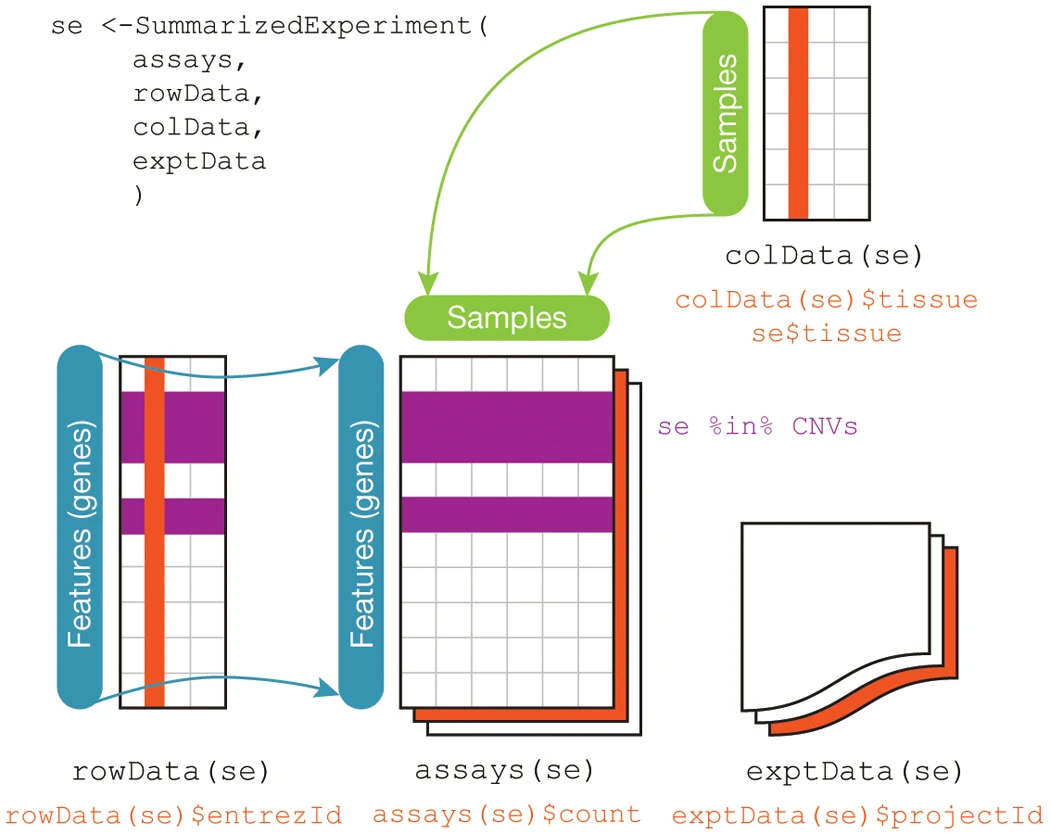
SummarizedExperiment Details
SummarizedExperimentclass is used ubiquitously throughout the Bioconductor package ecosystemSummarizedExperimentstores:- Processed data (
assays) - Metadata (
colDataandexptData) - Annotation data (
rowData)
- Processed data (