Project 3: ChIPseq
Now that we have experience with Nextflow from two prior projects, the
directions for this project will be much less detailed. I will describe what you
should do and you will be expected to implement it yourself. If you are asked to
perform a certain task, you should create working nextflow modules, construct
the proper channels in your main.nf, and run your workflow.
Please follow all the conventions we’ve established so far in the course.
These conventions include:
- Using isolated containers specific for each tool
- Write extensible and generalizble nextflow modules for each task
- Encoding reference file paths in the
nextflow.config - Encoding sample info and sample file paths in a csv that drives your workflow
- Requesting appropriate computational resources per job
Project 3 Workflow Diagram
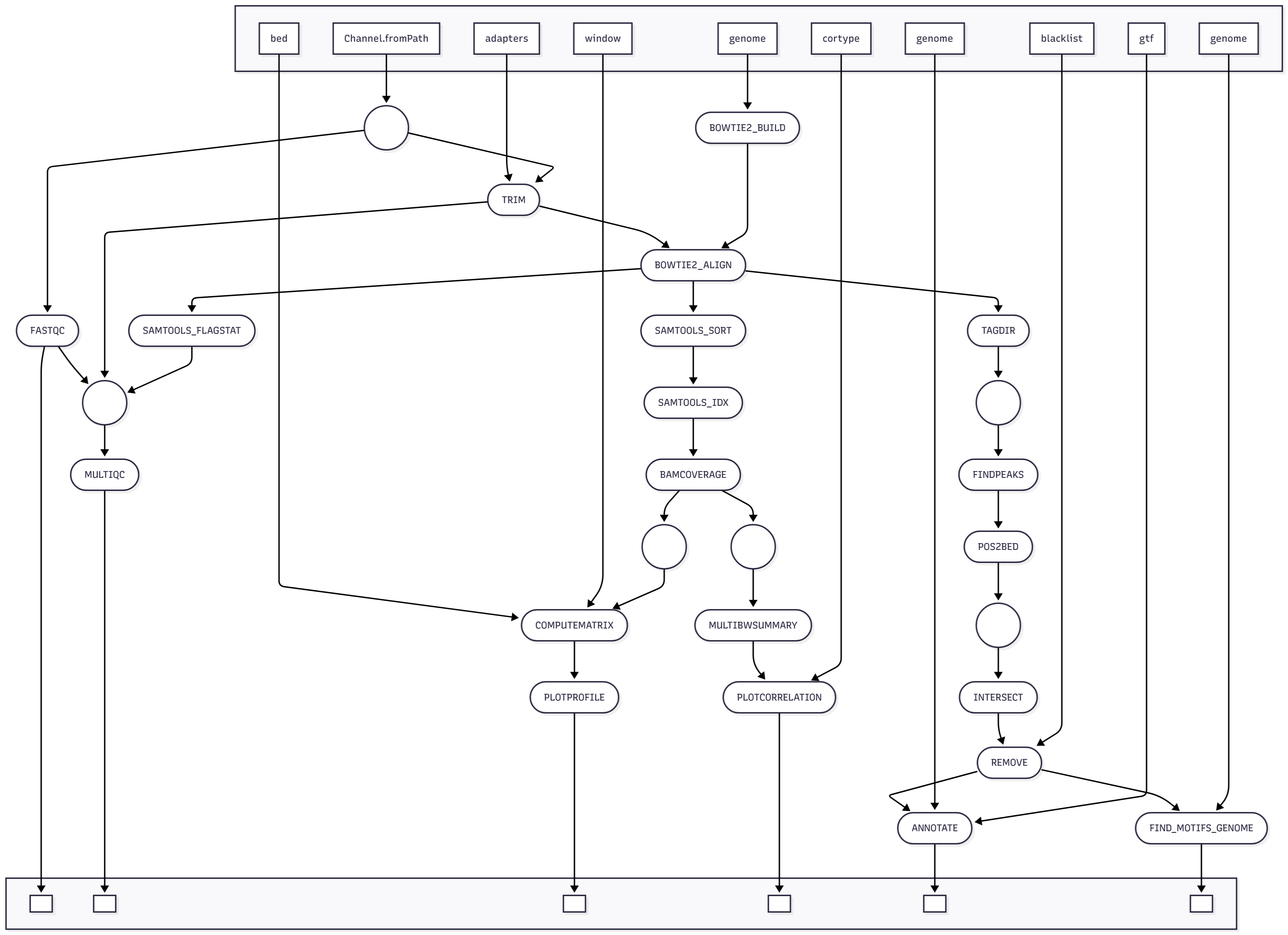
Containers for Project 3
FastQC: ghcr.io/bf528/fastqc:latest
multiQC: ghcr.io/bf528/multiqc:latest
bowtie2: ghcr.io/bf528/bowtie2:latest
deeptools: ghcr.io/bf528/deeptools:latest
trimmomatic: ghcr.io/bf528/trimmomatic:latest
samtools: ghcr.io/bf528/samtools:latest
bedtools: ghcr.io/bf528/bedtools:latest
homer/samtools: ghcr.io/bf528/homer_samtools:latest
Week 1: ChIPseq
Overview
This was a ChIPseq experiment from human cell lines that generated two replicates. This works out to four files per sample (two for IP and two for INPUT). The replicates are paired and denoted by the suffix _rep1 and _rep2. The IP and INPUT for each replicate originated from the same sample and should be used together when performing peak calling.
IP (Immunoprecipitate) refers to the reads for the factor of interest and INPUT refers to the reads for the control. The IP samples were the sequences enriched for binding for our factor of interest. INPUT is used to normalize the IP reads and allow us to make more robust inferences about enrichment of binding in the IP relative to what we expected in the background or INPUT.
For many NGS experiments, the initial steps are largely universal. We perform quality control on the sequencing reads, build an index for the reference genome, and align the reads. However, the source of the data will inform what quality metrics are relevant and the particular choice of tools to accomplish these steps. For RNAseq, it is important to use a splice-aware aligner when aligning against a reference genome since our sequences originated from mRNA. For ChIPseq experiments, our reads originated from DNA sequences and we can use a non-splice aware algorithm to map our reads to the reference genome.
Objectives
-
Assess QC on sequencing reads using FastQC
-
Trim adapters and low-quality reads using Trimmomatic
-
Align trimmed reads to the human reference genome
-
Run samtools flagstat to assess alignment statistics
-
Use MultiQC to aggregate all of the QC metrics
-
Use samtools to sort and index your BAM (alignment) files
Quality Control, Genome indexing and alignment
Between the past projects and the early labs we did, you should have working modules that perform quality control using FastQC and trimmomatic, build a genome index using bowtie2, and align reads to a genome. We are going to take advantage of the modularity of nextflow by simply copying these previous modules and incorporating them into this workflow.
The samples termed IP are the samples of interest (IP for a factor of interest) and the samples labeled INPUT are the control samples. Remember ChIP-seq experiments are paired (e.g. INPUT_rep1 is the control for IP_rep1)
- Use the provided CSV files that point to both the subsampled and full files. When you are developing the beginning of your workflow, use the subsampled files (they will not work once you get to the peak calling step). I have made the initial channel for you.
Please note that the subsampled_files are named differently than the full files!
-
The paths to the human reference genome, GTF and a few other critical files are already encoded in your
nextflow.config. -
Update your workflow
main.nfto perform quality control using FastQC and trimmomatic, build a bowtie2 index for the human reference genome and align the reads to the reference genome. Remember that we have worked on code for bowtie2 build, bowtie2 align, multiqc, samtools sort, samtools index, and deeptools bamCoverage in labs.
N.B. Some of the code from the labs will need to be modified to work for this specific experiment (paired end vs. single end, etc.)
Sorting and indexing the alignments
Many subsequent analyses on our BAM files will require them to be both sorted and indexed. Just like for large sequences in FASTA files, sorting and indexing the alignments will allow us to perform much more efficient computational operations on them.
- Create a module(s) that will both sort and index your BAM files using Samtools.
Calculate alignment statistics using samtools flagstat
The samtools flagstat utility will report various statistics regarding the alignment flags found in the BAM.
- Create a module that will run samtools flagstat on all of your BAM files
Aggregating QC results with MultiQC
Just like in project 2, we are going to use multiqc to collect the various quality control metrics from our pipeline. Ensure that multiqc collects the outputs from FastQC, Trimmomatic and flagstat.
-
Make a channel in your workflow
main.nfthat collects all of the relevant QC outputs needed for multiqc (fastqc zip files, trimmomatic log, and samtools flagstat output) -
Copy your previous multiqc module and incorporate it into your workflow to generate a MultiQC report for the listed outputs
Generating bigWig files from our BAM files
Now that we have sorted and indexed our alignments, we are going to generate bigWig files or coverage tracks containing the number of reads per genomic interval or bin for each sample. We will use these coverage tracks for calculating correlation between our samples and visualizing the read coverage in specific regions of interest.
-
Use the
bamCoveragedeeptools utility to generate a bigWig file for each of the sample BAM files. -
You may use all default parameters. If you wish, you may change the
-bsand-pflags as needed.
Week 1 Tasks Summary
-
Create nextflow modules that run the following tools:
- FastQC
- Trimmomatic
- Bowtie2 index
- Bowtie2 Align
- Samtools Sort
- Samtools Index
- Samtools Flagstats
- Deeptools bamCoverage
- MultiQC
-
Use the initial provided channel and params in the
nextflow.configand create a workflow that runs all of the modules in the correct order
Week 2: ChIPseq
Overview
For week 2, you will be performing a quick quality control check by plotting the correlation between the bigWigs you generated last week. Then, you will be performing standard peak calling analysis using HOMER, generating a single set of reproducible and filtered peaks, and annotating those peaks to their nearest genomic feature.
Objectives
-
Plot the correlation between the bigWig representations of your samples
-
Perform peak calling using HOMER on each of the two replicate experiments
-
Use bedtools to generate a single set of reproducible peaks with ENCODE blacklist regions filtered out
-
Annotate your filtered, reproducible peaks using HOMER
Plotting correlation between bigWigs
Recall that the bigWigs we generate represent the count of reads falling into various genomic bins of a fixed size quantified from the alignments of each sample. Assuming the experiment was successful, we naively expect that the IP samples should be highly similar to each other as they should be capturing the same binding sites for the factor of interest. Following this logic, the input controls which represent a random background of DNA from the genome should be different from the IP samples and somewhat more similar to each other.
We are going to perform a quick correlation analysis between the distances in our bigWig representations of our BAM files to determine the similarity between our samples with the above assumptions in mind.
-
Create a module and use the multiBigwigsummary utility in deeptools to create a matrix containing the information from the bigWig files of all of your samples.
-
Create a module and use the plotCorrelation utility in deeptools to generate a plot of the distances between correlation coefficients for all of your samples. You will need to choose whether to use a pearson or spearman correlation. In a notebook you create, provide a short justification for what you chose.
Peak calling using HOMER
In plain terms, peak calling algorithms attempt to find areas of enriched reads in a genome relative to background noise. HOMER is a commonly used tool that incorporates a Poisson model and other methodologies to make robust peak-finding predictions. Generate a nextflow module and workflow that runs HOMER
-
Generate a module that runs makeTagDirectory on each of your BAM files
- Generate a module that runs findPeaks on each of your tag directories
- Ensure that you specify the
-style factorflag correctly for the samples
- Ensure that you specify the
-
You will need to figure out how to pass both the IP and the Control sample for each replicate to the same command. i.e. callpeak should run twice (IP_rep1 and control_rep1) and (IP_rep2 and control_rep2) as ChIP-seq experiments have paired IP and controls. The rep1 samples were derived from the same biological material and is a biological replicate for the rep 2 samples. You will end up with two sets of peak calls, one for each replicate pair.
- HOMER generates a TXT file containing the peak outputs. Typically, we want to work with peaks in the BED format. Generate a nextflow module that uses the homer pos2bed.pl utility to convert the peak outputs to BED format.
Generating a set of reproducible peaks with bedtools intersect
We discussed various strategies for determining a set of “reproducible” peaks. For the sake of expedience, we will be performing a simple intersection to come up with a single set of peaks from this experiment. Please come up with a valid intersection strategy for determine a reproducible peak. Remember that this choice is subjective, so make a choice and justify it
Generate a nextflow module and workflow that runs bedtools intersect to generate a set of reproducible peaks.
-
Use the bedtools
intersecttool to produce a single set of reproducible peaks from both of your replicate experiments. -
In your created notebook, please provide a quick statement on how you chose to come up with a consensus set of peaks.
Filtering peaks found in ENCODE blacklist regions
In next generation sequencing experiments, there are certain regions of the genome that have been empirically determined to be present at a high level independent of cell line or experiment. These unstructured and anomalous regions are problematic for certain analyses (ChIPseq) and are considered to be signal-artifact regions and commonly stored in the form of a blacklist
The Boyle LAB as part of the ENCODE project have very kindly produced a list of these regions in some of the major model organisms using a standard methodology. This list is encoded as a BED file and is hosted by the Boyle Lab/ Please encode the path to the blacklist in your params, you may find the file in the refs/ directory under materials/ for project 2.
- Create a module that uses bedtools to remove any peaks that overlap with the blacklist BED for the most recent human reference genome. Generally speaking, you can remove a peak if it overlaps a blacklisted region by even 1bp as that is sufficiently close to consider it a signal-artifact region.
Annotating peaks to their nearest genomic feature using HOMER
Now that we have a single set of reproducible peaks with signal-artifact blacklisted regions removed, we are going to annotate our peaks by assigning them an identity based on their closest genomic feature. While we have discussed many caveats to annotating peaks in this fashion, it is a quick and exploratory analysis that enables quick determination of the genomic structures your peaks are located in and their potential regulatory functions. You may find the manual page for HOMER and this utility here
-
Create a module that uses
homerand theannotatePeaks.plscript to annotate your BED file of reproducible peaks (filtered to remove blacklisted regions). -
You should directly provide both a reference genome FASTA and the matching GTF to use custom annotations. Look further down the directions page for the argument order. This will make use of your params for the reference fasta and the GTF.
Week 2 Tasks Summary
-
Create nextflow modules and a script that performs the following tasks:
- Create a correlation plot between the sample bigWigs using deeptools multiBigWigSummary and plotCorrelation
- Create a module that uses HOMER makeTagDirectory on each of your BAM files
- Use HOMER findPeaks to perform peak calling on both replicate experiments
- Generate a single set of reproducible peaks using bedtools
- Filter peaks contained within the ENCODE blacklist using bedtools
- Annotate peaks to their nearest genomic feature using HOMER
Week 3: ChIPseq
Overview
In week 3, you will be using the UCSC table browser to obtain a BED file containing the start and end positions of every gene in the HG38 human reference genome. This will enable you to plot the signal coverage from your samples in relation to genic structure (Transcription Start Site and Transcription Termination Site). You will also be performing motif enrichment to determine what motifs appear to be enriched in the binding sites detected in your peaks.
Objectives
-
Extract the TSS and TTS for every gene in the hg38 reference in BED format using the UCSC table browser
-
Use the deeptools utilities computeMatrix and plotProfile, the UCSC BED, and your IP sample bigwigs to create a signal intensity plot
-
Perform motif enrichment on your reproducible and filtered peaks using HOMER
Create and use a single Jupyter notebook for any images, reports or written discussion
Please create a single jupyter notebook (.ipynb) that contains all of the
requested figures, images or discussion requested. As in the previous projects, please
create a dedicated .yml file that specifies any needed packages (including
an up-to-date installation of ipykernel). You may refer to the website for
instructions on how to do this.
This will enable your notebook to utilize the conda environment described in that yml file and ensure that your analysis is done in a reproducible and potentially portable manner.
Download a HG38 gene BED from UCSC table browser
We will be creating a plot which will provide a quick visualization of the average signal across the gene body of all genes. We will scale every gene to a uniform size and display the counts of alignments falling in the annotated regions of the gene. This will allow us to quickly visualize at a very high-level where we see the majority of binding for our factor of interest.
To do this, we have already generated our bigWig files, but we will require the genomic coordinates of all of the genes in the reference genome. We will be using the UCSC table browser to extract out this information.
Navigate to the UCSC Table Browser, use the following settings to extract a BED file listing the TSS/TTS locations for every gene in the reference genome:
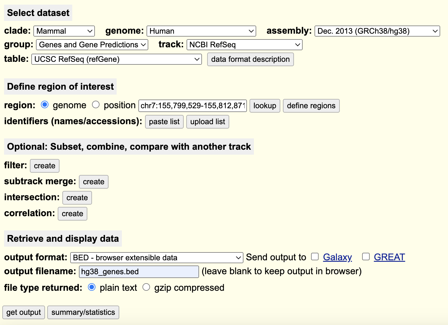
On the following page, do not change any options and you will be prompted to download a BED file containing the requested information. Ensure that you select the radio button for “Genome” and not “Position” so that your BED files has the chromosome, start, and end positions of every gene in the reference genome and not a selected region.
1. Put this BED file into your `refs/` working directory on SCC.
I have also provided this bed file in the materials/ directory for project 3.
This is a simple use case, but the UCSC table browser and UCSC genome browser are incredibly powerful tools and repositories for genome-wide sequencing data.
Generating a signal intensity plot for all human genes using computeMatrix and plotProfile for IP samples
Now that we have our bigWig files (count of reads falling into bins across the genome) and the BED file of the start and end position of all of the genes in the hg38 reference, we will calculate and visualize the signal falling into these annotated regions.
-
Use the
computeMatrixutility in deeptools, your bigWig files, and the BED file you downloaded to generate a matrix file containing the counts of reads falling into the regions in the bed files. -
Ensure that you use the scale-regions mode, and you specify the options to add 2000bp of padding to both the start and end site.
-
We are not interested in visualizing the input samples (which should represent random background noise), use an appropriate nextflow operator to ensure this is only done for the IP samples.
-
Use the outputs of
computeMatrixfor theplotProfilefunction and generate a simple visualization of the read counts from the IP samples across the body of genes from the hg38 reference.
Finding enriched motifs in ChIP-seq peaks
We will be using the single set of reproducible and filtered peaks from last week to search for enriched motifs in our peaks. Many DNA binding proteins have been found to have higher affinity for specific DNA binding sites with recurring sequence and pattern. These motifs may reveal key information about gene regulation by allowing for determination of what factors are binding in peaks. Remember that many DNA binding proteins bind as part of much larger multi-protein complexes that work in tandem to regulate gene expression. We will be using the HOMER tool to perform motif enrichment, you may find the manual here
- Use the
findMotifsGenome.plutility in homer to perform motif enrichment analysis on your set of reproducible and filtered peaks.
Week 3 Tasks Summary
-
Use the UCSC table browser to generate a BED file containing the TSS and TTS positions of every gene in the HG38 reference
-
Create nextflow modules and update your script to perform the following tasks:
-
Runs computeMatrix to generate a matrix containing the read coverage relative to the gene positions in the BED file
-
Uses plotProfile to visualize the results generated by computeMatrix for each of the two IP samples
-
Utilizes HOMER to perform basic motif finding on your reproducible and filtered peaks
-
Week 4: ChIPseq
Overview
For the final week, you will be reading the original paper and interpreting your results in the context of the publication’s results. Specifically, you will be focusing on reproducing the results shown in figure 2 with your own findings. This exercise is not meant to make any assertions as to the ground “truth” but to encourage you think about reproducibility in science.
Reminder
The tasks for this week will largely ask you to re-create the same figures found in the original publication with your own results. Remember that this is not meant to assert that one approach or one set of results are the only right answer. In science, we are constantly making assumptions and subjective choices, ideally based on sound logic and past knowledge, that will greatly impact the interpretation of the results we obtain. The purpose of this exercise is to explore the factors that contribute to reproducibility in bioinformatics and develop an understanding of what it means for an experiment or publication to be “reproducible”.
Objectives
-
Read the original publication and focus specifically on the results and discussion for figure 2
-
Reproduce figures 2D, 2E and 2F from the paper
-
Compare other key findings to the original publication
Read the original paper
The original publication has been posted on blackboard. Please read through the paper with a particular focus on the ChIP-Seq experiment presented in figure 2.
Overlap your ChIPseq results with the original RNAseq data
In their publication find the link to their GEO submission. Read the methods section of the paper and integrate your called ChIPSeq peaks with the results from their differential expression RNAseq experiment. Use your set of reproducible and filtered peaks, and use the publication’s listed significance thresholds for the RNAseq results.
-
You may do all of these steps in python using pandas or R using tidyverse / ggplot. You may start by reading the RNAseq results and the annotated peak results as dataframes.
-
Create a figure that displays the same information of figure 2F from the original publication using your annotated peaks and the RNAseq results. The figure does not have to be the same style but must convey the same information using your results.
-
In figures 2D and 2E, the authors identify and highlight two specific genes that were identified in both experiments. Using your list of filtered and reproducible peaks, a genome browser of your choice, and your bigWig files, please re-create these figures with your own results (You do not need to include the RNAseq data, but you should re-create the genomic tracks from your ChIPseq results)
-
In the notebook you created, please ensure you address the following questions:
-
Focusing on your results for figure 2f (You will likely not be able to exactly reproduce what they did - use the promoter-TSS start site in place of the gene body from your own results): - Do you observe any differences in the number of overlapping genes from both analyses? - If you do observe a difference, explain at least two factors that may have contributed to these differences. - What is the rationale behind combining these two analyses in this way? What additional conclusions is it supposed to enable you to draw?
-
Focusing on your results for figures 2D and 2E: - From your annotated peaks, do you observe statistically significant peaks in these same two genes? - How similar do your genomic tracks appear to those in the paper? If you observe any differences, comment briefly on why there may be discrepancies.
Comparing key findings to the original paper
Find the supplementary information for the publication and focus on supplementary figure S2A, S2B, and S2C.
- Re-create the table found in supplementary figure S2A. Compare the results with your own findings. Address the following questions:
-
Do you observe differences in the reported number of raw and mapped reads?
-
If so, provide at least two explanations for the discrepancies.
- Compare your correlation plot with the one found in supplementary figure S2B.
-
Do you observe any differences in your calculated metrics?
-
What was the author’s takeaway from this figure? What is your conclusion from this figure regarding the success of the experiment?
- Create a venn diagram with the same information as found in figure S2C.
-
Do you observe any differences in your results compared to what you see?
-
If so, provide at least two explanations for the discrepancies in the number of called peaks.
Analyze the annotated peaks
Use your annotated peaks list and perform an enrichment method of your choice. This is purposefully open-ended so you may consider filtering your peaks by different categories before performing some kind of enrichment analysis. There are a few peak / region based enrichment methods (GREAT) in addition to standard methods used such as DAVID / Enrichr.
-
In your created notebook, detail the methodology used to perform the enrichment.
-
Create a single figure / plot / table that displays some of the top results from the analysis.
-
Comment briefly in a paragraph about the results you observe and why they may be interesting.
Week 4 Detailed Tasks Summary
-
Read the original publication with a particular focus on figure 2
-
Write a methods section for the complete analysis workflow implemented by your pipeline while adhering to the guidelines and style discussed in class
-
Download the original publication’s RNAseq results and apply their listed significance threshold. Use this information to re-create figure 2F.
-
Re-create figures 2D and 2E and ensure you address the listed questions
-
Find supplementary figure S2 and re-create or compare your findings to supplementary figures 2A, 2B and 2C. Ensure you address any listed questions.
-
Perform an enrichment method using your annotated peaks and highlight the top results