Project 1: Genome Assembly
Project Overview
For this first project, you will be developing a nextflow pipeline to assemble a bacterial genome from long and short read sequencing data. You will be provided a scaffold of the nextflow pipeline and asked to implement the various steps outlined in the pipeline. You will not have to complete the entire pipeline, but will instead be asked to focus on various aspects of the workflow as we progress and get more comfortable with the tools and concepts. This project is broken up into weeks and each week will focus on different tasks. Future projects you will be working in a more open-ended manner and will be asked to implement the entire pipeline on your own.
For this week, you will be given a scaffolded nextflow pipeline and every week, we will continue to update and refine it until it resembles a final pipeline. The weeks after the first will include the previous week’s pipeline as well as additional improvements.
Week 1 - Understanding channels
As we will discuss in class, hybrid assembly approaches combine the benefits of both long and short read sequencing technologies. The long read sequencing provides improved contiguity and longer reads, which can better capture regions of the genome previously difficult to sequence using short reads. This is especially useful during genome assembly, where the longer reads are more likely to span all regions of the genome, greatly aiding in the assembly process. However, short reads are still useful and are commonly utilized to “polish” the assembly and remove systematic errors from the assembly of the long reads.
We will be generating a nextflow pipeline that will perform the following steps:
- Assembly of the nanopore reads
- Polishing of the nanopore assembly with the Illumina reads
- Quality Control of the polished assembly and comparison the reference genome
- Annotation of the genome and visualization of genomic features
Relevant Resources
- Nextflow Operators
- Nextflow Tutorial
- CLI Resources
- Computational Environments
- Basic Conda
- Nextflow Basics
- Nextflow Channels
Objectives
For the first week, we will focus on creating channels with the files we are going to process. You will also be asked to generate appropriate computational environments and look into the commands required to run certain tools. From a pipeline standpoint, we will be performing quality control on the short reads, quality control of the long reads, and then assembly of the long reads.
Setting up
For this week, I have provided you a fully working nextflow pipeline that will let you see how it works while focusing just on learning a few key concepts we will be using throughout the semester.
To start, open a VSCode session in your directory under the BF528 project
(i.e. /projectnb/bf528/students/<your_username>/). Please replace the
<your_username> with your BU ID and no @bu.edu. So if your BU ID was jstudent
then your directory would be /projectnb/bf528/students/jstudent/
Remember to activate the conda environment you created for nextflow using the following commands:
module load miniconda
conda activate nextflow_latest
- Please clone the github repo for this project in your student folder - you may find the link on blackboard. In your student directory, you may use the following command to clone your repo after copying the SSH link from your repo made for you on GitHub Classroom:
git clone <repo_url>
This will make clone the repo to your student directory and all of your work for this week should be done in this directory. You will push your changes to GitHub as you go, which will also enable us to evaluate your work and help troubleshoot.
-
Open this directory in your VSCode session.
-
Familiarize yourself with the directory you are working in. Throughout the semester, we will be using the same structure and organization in all of the projects.
Tasks
Creating a channel from a CSV file
- Take a look at the channel_test.nf and run the following command in a terminal with your nextflow environment active:
nextflow run channel_test.nf
-
Note what the output of the command is in your terminal window and remember what we talked about in class about channels and tuples.
-
Use the code in the channel_test.nf as an example and in the week1.nf, make two channels that are a tuple containing the name of the sample and the path to the long reads and short reads, respectively. Name the channels
longread_chandshortread_ch, respectively. Since we have paired-end sequencing for the short reads, the shortread_ch will be a tuple consisting of three elements while the longread_ch will be a tuple with only two elements.
If you view() the contents of these channels, they should look something like below (the paths will be different from what you see below and the actual paths will be their location on the SCC):
longread_ch
[Alteromonas_macleodii, /path/to/long_reads]
shortread_ch
[Alteromonas_macleodii, /path/to/short_reads1, /path/to/short_reads2]
These are both tuples where the first element is our sample identifier, and the remaining elements are the paths to the files we want to process.
Feel free to modify the code in the channel_test.nf and run it to view the
contents of the channels as you’re troubleshooting the logic to generate the
shortread_ch and longread_ch correctly.
Specifying appropriate computational environments
This pipeline is fully specified in the week1.nf file, but you will need to specify the appropriate computational environments for each process. In general, we will endeavor to always use the most up-to-date version of a tool. In the envs/ directory, you will find empty conda environment files for each tool already created for you that you will need to complete.
- Use the appropriate conda command to find the most recent version of each tool available on bioconda and update the YML files accordingly. Keep in mind the following:
- The command is
conda search -c conda-forge -c bioconda <tool_name> - Use the most up-to-date version and specify it as so:
tool_name=<version>, which will normally look likesamtools=1.17. Conda will list all available versions and the most-up-to-date version will be the last one in the list and should be the numerically highest version.
-
Only specify a single version of a tool in each YML file. While you can specify multiple versions of a tool in a single YML file, we will try to minimize this as much as possible to avoid running into issues with conda being unable to resolve the dependencies.
-
Once you’ve filled in the YML files, add the relative path to the YML file for each process after the line that begins with
condain the process.
This will look something like below:
process EXAMPLE {
    label 'process_single'
    conda 'envs/<name_of_yml_file>.yml
    ...
}
Make sure to replace
Please note how the path is relative to where the week1.nf file is located.
Finding the appropriate commands for running each tool
You’ll notice that the script block in each of the processes in the week1.nf
are blank. You will need to find the appropriate commands for running each tool
and fill them in.
There are several ways to figure out the appropriate commands for running each tool.
-
In an environment where you have the tool installed, you can use the help flag, which is usually
-hor--helpto see the appropriate command for running the tool. i.e.tool_name -hortool_name --help -
Many of the well-supported tools host either a GitHub repository or a wiki page where you can find the appropriate commands for running the tool as well as examples of how to use the tool. They will often have a
Usagesection that contains a quick basic example of how to use the tool. -
For FastQC and filtlonger, you may use the quick start command provided in the documentation. For filtlonger, choose the command for running without an external reference.
-
For Flye, the only arguments you should include in the command are
--nano-hqand the ‘-o .’ to specify the output directory.
A few hints:
- You will need to specify FASTQC to run on both the short read files (R1 and R2) by listing them one after another
- You can refer to files or variables passed in inputs using the
$symbol. i.e.$read1or$read2 - You can make strings by using string interpolation “${variable_name}.txt” will create a string using the value of the variable_name variable - i.e. if variable_name is “test”, then “${variable_name}.txt” will create the string “test.txt”.
- The file created by the tool should be specified in the
outputblock of the process.
Once you have found the appropriate commands for running each tool, you will need
to fill in the script block in each process in the week1.nf file.
When you believe you’ve finished this step, run the pipeline and observe if it runs successfully. If it doesn’t, you will need to go back and fix the commands for running each tool.
You may use the following command to run the pipeline:
nextflow run week1.nf -profile cluster,conda
Please note that if successful, this command may take around ~1 hour to run as Flye is performing assembly using the long reads, which as we discussed, is a computationally intensive process. Make sure not to end your VSCode interactive session while the pipeline is running. You can however close your browser window and your session will continue to run.
Week 1 Recap
- Clone the github repo for this project
- Familiarize yourself with the directory you are working in
- Use the code in the channel_test.nf to create two channels from a CSV file in your week1.nf
- Specify the appropriate computational environments for each process in the YML file and add the path to each YML file in the appropriate process
- Find the appropriate commands for running each tool and fill them in
- Run the pipeline and observe if it runs successfully
Week 2 - Modularizing our pipeline and polishing our assembly
You may have noticed from the first week that our pipeline is becoming increasingly complex and slightly onerous to read in a single file. In this week, we are going to refactor our workflow to make it more modular and easier to read. This modularity will have the secondary benefit of enabling us to reuse components of the pipeline in future projects or even share them with others.
From a bioinformatics standpoint, this week we will add several steps to our pipeline. We will first generate a genome index from the assembly and align the illumina reads to the draft assembly using bowtie2. We can then sort the aligned reads and provide them to Pilon to polish the assembly and fix any potential errors.
Relevant Resources
Objectives
For this week, you will again be given a working pipeline but this time, I will ask you to focus on connecting the processes by filling out the nextflow workflow. You will need to look at the inputs and outputs of the processes, and connect them appropriately.
Setting up
- Clone the github repo for this project - you may find the link on blackboard
Tasks
Ensure you are always running nextflow with -profile conda,cluster
Last week you were asked to run the pipeline with the conda and cluster profiles.
If you look in the nextflow.config file, you’ll notice that we have profiles
corresponding to these labels and a set of options specified. These options will
be automatically applied when you run the pipeline with the specified profile.
As we talked about in the lab, we will be using the SCC to run our pipelines and
nextflow will automatically submit each process as a separate job to the SCC using
the appropriate qsub commands when specified.
This week, we will be running significantly more resource intensive processes and we will need to now make use of the resource available to us on the SCC. You will be asked to determine the most appropriate set of resources for each of your processes.
As a reminder, you should run your pipelines with the following command:
nextflow run main.nf -profile cluster,conda
Keep in mind that this will submit each of your processes as separate jobs to different compute nodes on the cluster. This may take significantly longer to run as your job will potentially need to wait in the queue for resources to become available, processes may also take longer as they are more complex and certain processes may need to wait until others finish.
Modularize the remaining processes in the week2.nf
Before you begin, take note of the week2.nf file you’ve been provided and the
modules/ directory. If you’ve been following along, you’ll notice that we’ve
changed how we have organized our pipeline. The same code from our week 1 pipeline
is there, but we have now separated each process into a different module located
in a named directory in modules/. This allows us to remove the processes from the
week2.nf file and import them into the week2.nf file using the include keyword.
You can think of this as akin to when you import a library in python to make
certain functions available for use.
- Take the code for the processes BOWTIE2_INDEX, BOWTIE2_ALIGN, SAMTOOLS_SORT,
and PILON found in the week2.nf and separate them out into modules the
way I have already done for you with last week’s code. You should remove this
code from the
week2.nffile and place them in new text files following the same format as last week’s modules. When finished, your week2.nf should begin with the INCLUDE statements and end with the workflow block.
- Follow the same pattern where you make a new directory in modules/ with the name of the process and the file itself called main.nf.
- Just as I’ve done for you with last week’s processes, at the top of your
week2.nf file before the
workflowblock, you should use theincludekeyword to import the processes you have created new modules for. Follow the same syntax and style that is already there.
Workflow directed acyclic graph (DAG)
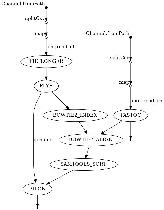
Connect the processes in the week2.nf
- Look at the inputs and outputs of each module and try to construct the workflow by passing the correct channels to each process. You will need to understand the order of operations and the dependencies between the processes to construct the workflow. If you find it useful, I have included a visual representation of the DAG for the workflow in these directions and in your repository. You should add the processes to the workflow in the order they should be run and with the right dependencies. A dependency in this context is simply a process that must be run and finish before the next process can begin.
- Remember that you may access the outputs of a process using the
.out() notation. For example, if you have a process called `FASTQC`, you can access the output of the process using `FASTQC.out()`. If you have named different outputs, you refer to them by the named defined in the `emit` block of the process. For example, if you have a process called `FASTQC` that emits two different output channels called `html` and `zip`, you can access them using `FASTQC.out.html` and `FASTQC.out.zip`.
If you complete this successfully, you should have a working pipeline that should run last week’s tasks as well as the steps from this week that will assemble the reads, align the short reads to the assembly, sort the alignments, and use the short reads to polish the assembly.
You’ll notice that when we go to align reads to the reference sequence, we first have to build an index. We will discuss more in-class about this step, but essentially, most aligners need to build a data structure that allows them to quickly and efficiently align reads to the reference sequence and locate where they align. You can think of a genome index as akin to a table of contents, which allows you to determine what page a chapter is located on, without having to read through the entire book. Most traditional aligners will need to build an index for the reference sequence before they can align reads to it, and most indexes need to be built with the same tool as the aligner.
Before you run the pipeline, please complete the following section.
Use the report and the list of SCC resources to give each process an appropriate label
In the repo, I have provided you a HTML report that can be obtained from running
nextflow with the -with-report flag (i.e. nextflow run week2.nf -profile cluster,conda -with-report).
This report shows you the amount of resources used per process. Use this information
and the guide for requesting SCC resources
to give each process an appropriate label.
-
Look at the report and try to give each process an appropriate label. Focus on the amount of VMEM (virtual memory) required for each task and ensure that your label requests the appropriate amount of RAM. You want to look at the virtual memory usage tab of the memory section in the report. See here for more details.
-
Edit your
nextflow.configto add the appropriate label specifications. I have provided you a sample label in the config file that you can use as a model for the ones you create. Please create labels calledprocess_low, andprocess_mediumthat specify a different number of CPUs to request.
You can see an example of where I’ve added a label to a process in the FLYE
process. You’ll also notice that in the command, I have to specify the option
specific to FLYE for using multiple threads, -t and I use the $task.cpus
variable in nextflow to automatically fill in the number of cpus requested for
the selected label. If you look in the nextflow.config, you can see that the
label ‘process_high’ requests 16 cpus, which also reserves 128GB of memory.
- For the other processes, please specify an appropriate label like in the FLYE
process and ensure you add the right flag to each command to make use of the resources
requested. You will need to use the
$task.cpusvariable in nextflow to automatically fill in the number of cpus requested for the selected label in the command as well as find the right flag to use for each tool by looking at their documentation.
-
Certain processes like building an index or aligning reads to the reference benefit greatly from using multiple threads / cores. You can use a higher number of threads / cores for these processes if you have the resources available and it will greatly speed up the process. You may choose to use a greater number of threads for these processes even if you don’t technically need more memory reserved.
-
Some tools may not be able to use multiple threads / cores, but you should still use the provided report to specify an appropriate label so that your job properly reserves the right amount of memory.
Week 2 Recap
- Modularize the remaining processes in the week2.nf
- Connect the processes in the week2.nf
- Create labels in your nextflow.config for
process_lowandprocess_medium - Use the report and the list of SCC resources to give each process an appropriate label - ensuring that each process has requested a node with enough memory.
- Run the pipeline and observe if it runs successfully
Week 3 - Wrapping up and evaluating our assembly
For the final week, we will be evaluating our assembly and comparing it to a reference genome. As we briefly discussed in class, there are several important criteria we can use to evaluate our assembly, including contiguity, completeness and correctness. We will be performing several analyses to look at the quality of our genome.
Relevant Resources
Objectives
As with last week, I will provide you working modules and task you with connecting them to form a working pipeline. Please focus on understanding how inputs and output channels are passed between processes and how to connect them appropriately. I will ask you to put together a single nextflow process to run prokka. You will have to determine the right inputs and outputs as well as the appropriate running command. You will once again be provided a visual diagram of the workflow and you will need to figure out the order of operations and dependencies between the processes to construct the workflow.
You should also use the remaining time to put together your writeup for project 1 if you haven’t already.
Setting up
- Clone the github repo for this project - you may find the link on blackboard
Tasks
Workflow Visualization - DAG

Connect the processes
-
Look at the inputs and outputs of each module and try to construct the workflow by passing the correct channels to each process. You will need to understand the order of operations and the dependencies between the processes to construct the workflow. If you find it useful, I have included a visual representation of the DAG for the workflow in these directions and in your repository. Please note that while you can alter the inputs / outputs, you should be able to run the pipeline successfully by simply passing the correct outputs to the correct processes. If you do change the inputs / outputs, you will need to ensure that the pipeline still runs successfully.
-
Run the pipeline and observe if it runs successfully. If it doesn’t, you will need to go back and fix the workflow.
You should use the following command:
nextflow run main.nf -profile cluster,conda
Finalize the project report for project 1
Follow the Project 1 Report Guidelines to make a final report for this project.
Week 3 Recap
- Connect the processes
- Finalize the project report for project 1